Co-translational exoribonucleolytic degradation profiling in S. aureus using 5’ end RNA-Seq data
Complete source of this page is available in the notebook Degradation_profiling.Rmd.
library(tidyverse)
time_start <- now()
library(ggpubr)
library(rnaends)
Co-translational exoribonucleolytic degradation analysis using 5’ end RNA-Seq data
Based on the publication from Khemici V, Prados J, Linder P, Redder P (2015) Decay-Initiating Endoribonucleolytic Cleavage by RNase Y Is Kept under Tight Control via Sequence Preference and Sub-cellular Localisation. PLoS Genetics, 11. https://doi.org/10.1371/journal.pgen.1005577.
Download datasets
Data from this article are available on Gene Expression Omnibus (GEO) database: GSE68811
For this notebook, we will only use 4 RNA-Seq samples corresponding to 4 EMOTE assays on Staphylococcus aureus SA564 strain (GSM1682239, GSM1682240, GSM1682241, GSM1682242).
We download data directly in a the “extdata” directory of the GitLab project in the sub-directory called “RNaseY_Khemici” where the reference genome and the genome annotation files are already provided when the project is cloned.
options(timeout = 3600)

list_SRR = c("SRR2017583", "SRR2017584", "SRR2017585", "SRR2017586")

for (i in list_SRR){
    raw_fastq = paste0("../extdata/RNaseY_Khemici/", i, ".fastq.gz")
    if (!file.exists(raw_fastq))
        download.file(paste0("https://trace.ncbi.nlm.nih.gov/Traces/sra-reads-be/fastq?acc=",i),
                      destfile = raw_fastq)
}
Pre-processing
Parse reads (+ read features)
In order to make reads mappable, we must remove the oligonucleotide that is still present at the 5’-end of the reads in the FASTQ files.
We use the function parse_read to remove this oligonucleotide and filter out reads for which the oligo does not contain all the expected elements. These reads have the same structure as in Prados et al. 2016 (https://bmcgenomics.biomedcentral.com/articles/10.1186/s12864-016-3211-3).
parse_reads requires a read_features table which describes each element that should be found in the reads.
Following the Material & Methods section of the article, reads are not trimmed and should look like this (X is the sequence of the 5’end of RNA to be mapped to the reference):
      1       2            5      6            20     21    27      28 30     31                  50
      N     - (EMOTE barcode) -   CGGCACCAACCGAGG    - VVVVVVV -     CGC     - XXXXXXXXXXXXXXXXXXXXX
1 random nt -  EMOTE barcode  -   recognition.seq    -   UMI   - control.seq -     RNA 5'-end
We need to keep only the “RNA 5’-end” part that should map on the reference genome.
init_read_features and add_read_feature functions are used to create a read_features table which specifies the read structure.
The initialization of the read_features table is initialized with the init_read_features function because the minimum read_features table contains the readseq feature (i.e. the mappable part to keep in the FASTQ file).
According to our scheme, the readseq part begins at nucleotide 31 and is 20 nucleotides long (Illumina50).
rf <- init_read_features(start = 31, width = 20)
We add other features such as barcode which begins at position 2 and is 4 bases long.
For the pattern parameter, we specify the authorized barcode sequences to validate the feature (here we allowed 1 out of 4 sequences).
We use the pattern_type parameter to specify the type of pattern we seek: “constant” means that we query the exact character string provided in the pattern parameter allowing n number of mismatches (specified by the max_mismatch parameter).
Finally, the readid_prepend parameter is used to specify if the feature retrieved should be stored in the read identifier (1st line of a read records in the FASTQ file). It may be useful to keep the information of the sequence found of a feature since they are removed and therefore absent from the FASTQ output file.
rf <- add_read_feature(rf,
                       name = "barcode",
                       start = 2,
                       width = 4,
                       pattern_type = "constant",
                       pattern = c("GTAT","CAAG","TACA","TCGG"),
                       readid_prepend = FALSE)
The recognition sequence feature begins at position 6 and is 15 bases long. We expect a single unique sequence with maximum 1 mismatch:
rf <- add_read_feature(rf,
                       name = "Recog. seq",
                       start = 6,
                       width = 15,
                       pattern_type = "constant",
                       pattern = "CGGCACCAACCGAGG",
                       max_mismatch = 1,
                       readid_prepend = FALSE)
The UMI feature begins at position 21 and is 7 bases long.
UMIs are random nucleotide sequences. Thus, the patern_type is set to “nucleotides”. It it possible to provide a list of expected characters (here A, C or G).
We set readid_prepend = TRUE. This is mandatory as we will need the UMI associated to the 5’-end RNA during the quantification to remove PCR duplicates.
Note: the readseq feature has the same pattern_type than UMI which is set by default to A, T, C or G random sequence.
rf <- add_read_feature(rf,
                       name = "UMI",
                       start = 21,
                       width = 7,
                       pattern_type = "nucleotides",
                       pattern = "ACG",
                       max_mismatch = 0,
                       readid_prepend = TRUE)
The control sequence feature begins at position 28 and is 3 bases long. We expect a specific sequence (pattern_type = "constant").
rf <- add_read_feature(rf,
                       name = "Control seq.",
                       start = 28,
                       width = 3,
                       pattern_type = "constant",
                       pattern = "CGC",
                       max_mismatch = 0,
                       readid_prepend = FALSE)
The final read_features table describing the read structure is as follows:
rf %>%
  arrange(start) %>%
  knitr::kable()
name |
start |
width |
pattern_type |
pattern |
max_mismatch |
readid_prepend |
|---|---|---|---|---|---|---|
barcode |
2 |
4 |
constant |
GTAT, CA…. |
0 |
FALSE |
Recog. seq |
6 |
15 |
constant |
CGGCACCA…. |
1 |
FALSE |
UMI |
21 |
7 |
nucleotides |
ACG |
0 |
TRUE |
Control seq. |
28 |
3 |
constant |
CGC |
0 |
FALSE |
readseq |
31 |
20 |
nucleotides |
ACTG |
0 |
FALSE |
Now, we can use the parse_reads function on the 4 FASTQ files using the read_features table as parameter.
lapply(
    list.files("../extdata/RNaseY_Khemici", pattern = ".fastq.gz$", full.names = TRUE),
    FUN = parse_reads,
    yieldsize = 5e6, # Number of reads parsed at each iteration
    features = rf, # The features table
    out_dir = "../extdata/RNaseY_Khemici/parse_results",
    keep_invalid_reads = FALSE, # We don't want to store invalid reads
    force = TRUE,
) %>%
  bind_rows() %>%
  head(15) %>%
  knitr::kable()
is_valid_readseq |
is_valid_barcode |
is_valid_Recog. seq |
is_valid_UMI |
is_valid_Control seq. |
count |
|---|---|---|---|---|---|
FALSE |
FALSE |
FALSE |
FALSE |
FALSE |
7 |
FALSE |
FALSE |
FALSE |
TRUE |
FALSE |
25 |
FALSE |
FALSE |
FALSE |
TRUE |
TRUE |
2 |
FALSE |
FALSE |
TRUE |
FALSE |
FALSE |
12 |
FALSE |
FALSE |
TRUE |
TRUE |
FALSE |
43 |
FALSE |
TRUE |
TRUE |
FALSE |
FALSE |
5404 |
FALSE |
TRUE |
TRUE |
FALSE |
TRUE |
696 |
FALSE |
TRUE |
TRUE |
TRUE |
FALSE |
16155 |
FALSE |
TRUE |
TRUE |
TRUE |
TRUE |
17331 |
TRUE |
FALSE |
FALSE |
FALSE |
FALSE |
3294 |
TRUE |
FALSE |
FALSE |
FALSE |
TRUE |
50 |
TRUE |
FALSE |
FALSE |
TRUE |
FALSE |
16606 |
TRUE |
FALSE |
FALSE |
TRUE |
TRUE |
154 |
TRUE |
FALSE |
TRUE |
FALSE |
FALSE |
4571 |
TRUE |
FALSE |
TRUE |
FALSE |
TRUE |
61 |
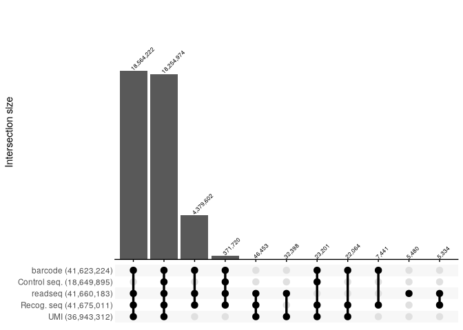
parse_reads returned a table which contains some information on the features validity.
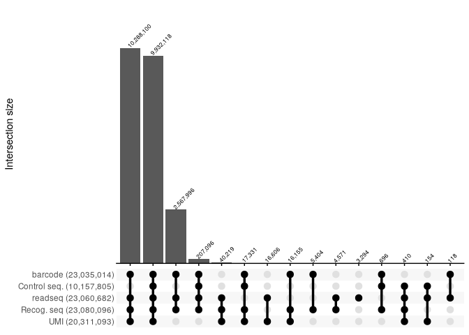
Upset plots for each raw original FASTQ file.
report_SRR2017583 <- read_csv("../extdata/RNaseY_Khemici/parse_results/SRR2017583_parse_report.csv", show_col_types = FALSE)

report_SRR2017583 %>%
  filter(count >=100) %>%
  reads_parse_report_ggupset(margin=0.2)
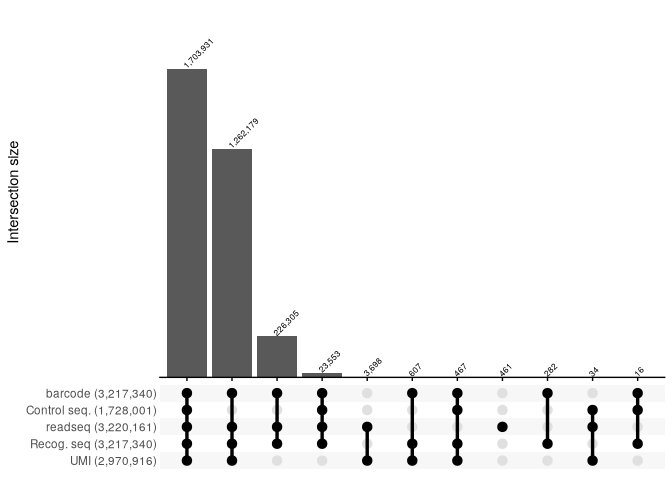
report_SRR2017584 <- read_csv("../extdata/RNaseY_Khemici/parse_results/SRR2017584_parse_report.csv", show_col_types = FALSE)

report_SRR2017584 %>%
  filter(count >=10) %>%
  reads_parse_report_ggupset(margin=0.2)
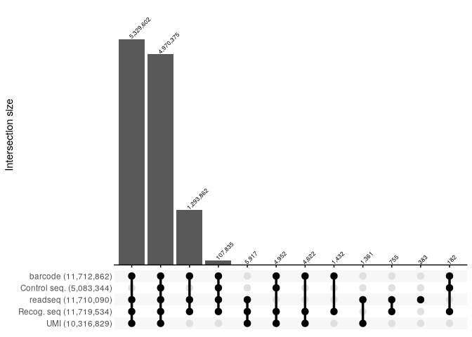
report_SRR2017585 <- read_csv("../extdata/RNaseY_Khemici/parse_results/SRR2017585_parse_report.csv", show_col_types = FALSE)

report_SRR2017585 %>%
  filter(count >=100) %>%
  reads_parse_report_ggupset(margin = 0.15)
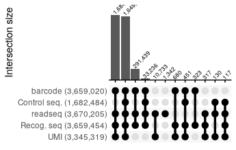
report_SRR2017586 <- read_csv("../extdata/RNaseY_Khemici/parse_results/SRR2017586_parse_report.csv", show_col_types = FALSE)

report_SRR2017586 %>%
  filter(count >=100) %>%
  reads_parse_report_ggupset(margin = 0.15)
All repotrs combined:
report_SRR2017583 %>%
  bind_rows(report_SRR2017584) %>%
  bind_rows(report_SRR2017585) %>%
  bind_rows(report_SRR2017586) %>%
  group_by(across(starts_with("is_valid_"))) %>%
  summarise(count = sum(count), .groups = "drop") %>%
  filter(count>5000) %>%
  reads_parse_report_ggupset(angle = 45, margin=0.35)
Quantification
Mapping
Reads are now ready to be aligned on the reference genome using the map_fastq_files function.
Note: a single FASTQ file can be mapped with the map_fastq function.
bf <- map_fastq_files(
  list_fastq_files = list.files("../extdata/RNaseY_Khemici/parse_results",
                                pattern = "_valid.fastq.gz$",
                                full.names = TRUE) ,
  index_name = "../extdata/RNaseY_Khemici/CP010890.bt", # Path of the genome index (created if not exists)
  fasta_name = "../extdata/RNaseY_Khemici/CP010890.fasta", # Path of the reference genome file
  bam_dir = "../extdata/RNaseY_Khemici/mapping_results", # Output directory
  max_map_mismatch = 1,
  aligner = "bowtie", # Either bowtie or subread
  map_unique = TRUE,
  force = TRUE,
  threads = 3
)
#> Warning in FUN(X[[i]], ...): Index directory already exists remove it if you
#> want to recreate it
#> Warning in FUN(X[[i]], ...): Index directory already exists remove it if you
#> want to recreate it
#> Warning in FUN(X[[i]], ...): Index directory already exists remove it if you
#> want to recreate it
#> Warning in FUN(X[[i]], ...): Index directory already exists remove it if you
#> want to recreate it
bf
#> [[1]]
#> [1] "../extdata/RNaseY_Khemici/mapping_results/SRR2017583_valid.fastq.gz.bam"
#>
#> [[2]]
#> [1] "../extdata/RNaseY_Khemici/mapping_results/SRR2017584_valid.fastq.gz.bam"
#>
#> [[3]]
#> [1] "../extdata/RNaseY_Khemici/mapping_results/SRR2017585_valid.fastq.gz.bam"
#>
#> [[4]]
#> [1] "../extdata/RNaseY_Khemici/mapping_results/SRR2017586_valid.fastq.gz.bam"
Mapping statistics
Use the map_stats_bam_files function to get some basic statistics on the mapping we’ve just made:
map_stats_bam_files(bam_files = bf) %>%
  knitr::kable()
#> BAM file mapping stats exists '../extdata/RNaseY_Khemici/mapping_results/SRR2017583_valid.fastq.gz.bam.map_stats.csv' already exists, set force=TRUE to recompute
#> BAM file mapping stats exists '../extdata/RNaseY_Khemici/mapping_results/SRR2017584_valid.fastq.gz.bam.map_stats.csv' already exists, set force=TRUE to recompute
#> BAM file mapping stats exists '../extdata/RNaseY_Khemici/mapping_results/SRR2017585_valid.fastq.gz.bam.map_stats.csv' already exists, set force=TRUE to recompute
#> BAM file mapping stats exists '../extdata/RNaseY_Khemici/mapping_results/SRR2017586_valid.fastq.gz.bam.map_stats.csv' already exists, set force=TRUE to recompute
bam_file |
mapped |
unmapped |
pc_mapped |
|---|---|---|---|
SRR2017583_valid.fastq.gz.bam |
1785951 |
1147874 |
60.87 |
SRR2017584_valid.fastq.gz.bam |
585774 |
210122 |
73.60 |
SRR2017585_valid.fastq.gz.bam |
999717 |
477088 |
67.69 |
SRR2017586_valid.fastq.gz.bam |
1074276 |
494215 |
68.49 |
Quantification (counts computation)
In order to obtain counts by position, we use the quantify_from_bam_files function to parse previously obtained BAM files in bf.
This function allows the quantification of either the 5’-ends (quantify_5prime) or the 3’-ends (quantify_3prime), in both cases, it is an exact position quantification.
For UMIs to be taken into account for the quantification, we provide the read_features table with the “features” parameter.
The keep_UMI parameter is used to record the number of copy of each UMI by exact position. This level of information is not nedded for this analysis and we use it as default (FALSE).
count_table <- quantify_from_bam_files(
    bam_files = bf,
    sample_ids = c("WT_rep1","WT_rep2","DY_rep1","DY_rep2"),
    fun = quantify_5prime, # Either quantify_5prime or quantify_3prime
    features = rf,
    keep_UMI = FALSE,
    force = TRUE)
count_table %>%
  head(15) %>%
  knitr::kable()
sample_id |
rname |
position |
strand |
reads |
count |
|---|---|---|---|---|---|
WT_rep1 |
CP010890.1 |
313 |
+ |
67 |
34 |
WT_rep1 |
CP010890.1 |
314 |
+ |
7 |
3 |
WT_rep1 |
CP010890.1 |
316 |
+ |
5 |
3 |
WT_rep1 |
CP010890.1 |
362 |
+ |
4 |
3 |
WT_rep1 |
CP010890.1 |
370 |
+ |
1 |
1 |
WT_rep1 |
CP010890.1 |
374 |
+ |
1 |
1 |
WT_rep1 |
CP010890.1 |
377 |
+ |
1 |
1 |
WT_rep1 |
CP010890.1 |
412 |
+ |
1 |
1 |
WT_rep1 |
CP010890.1 |
413 |
+ |
1 |
1 |
WT_rep1 |
CP010890.1 |
437 |
+ |
1 |
1 |
WT_rep1 |
CP010890.1 |
445 |
+ |
1 |
1 |
WT_rep1 |
CP010890.1 |
467 |
+ |
1 |
1 |
WT_rep1 |
CP010890.1 |
491 |
+ |
1 |
1 |
WT_rep1 |
CP010890.1 |
493 |
+ |
9 |
3 |
WT_rep1 |
CP010890.1 |
513 |
+ |
1 |
1 |
The above count table will allow us to perform some downstream analysis.
Note: here, the count column corresponds to the number of different UMIs mapped at this exact position. This is why it is lower or equal to the reads values (due to PCR duplicates).
Downstream analysis
Ribosome profilling
Note: the following functions can take BAM files as input instead of count table. In that case, additional parameters must be provided that correspond to the quantify_from_bam_files function parameters.
Annotation table preparation
In order to retrieve the number of reads mapped on the CDSs, we need to have access to the position (start and stop) of these CDSs.
We simply retrieved the annotation file of the reference strain SA564 from the NCBI that we filter to get only the feature corresponding to “CDS”.
Note: we also switch the positions for CDS on the reverse strand start and stop as their genomic positions are inverted.
annot <- read_tsv("../extdata/RNaseY_Khemici/CP010890.gff3",
                  show_col_types = FALSE,
                  col_names = c("chr",
                                "type",
                                "feature",
                                "begin",
                                "end",
                                "V1",
                                "strand",
                                "V2",
                                "annotation")) %>%
  filter(feature=="CDS") %>%
  mutate(start = ifelse(strand=="-" & begin<end, end, begin),
         end = ifelse(strand=="-" & begin<end, begin, end)) %>%
  select(chr, feature, strand, start, end, annotation)

annot %>%
  head(15) %>%
  knitr::kable()
chr |
feature |
strand |
start |
end |
annotation |
|---|---|---|---|---|---|
CP010890.1 |
CDS |
+ |
517 |
1878 |
ID=cds-ALD79596.1;Parent=gene-RT87_00005;Dbxref=NCBI_GP:ALD79596.1;Name=ALD79596.1;gbkey=CDS;inference=EXISTENCE: similar to AA sequence:RefSeq:WP_001290432.1;locus_tag=RT87_00005;product=chromosomal replication initiation protein;protein_id=ALD79596.1;transl_table=11 |
CP010890.1 |
CDS |
+ |
2156 |
3289 |
ID=cds-ALD79597.1;Parent=gene-RT87_00010;Dbxref=NCBI_GP:ALD79597.1;Name=ALD79597.1;gbkey=CDS;inference=EXISTENCE: similar to AA sequence:RefSeq:WP_000969809.1;locus_tag=RT87_00010;product=DNA polymerase III subunit beta;protein_id=ALD79597.1;transl_table=11 |
CP010890.1 |
CDS |
+ |
3679 |
3915 |
ID=cds-ALD79598.1;Parent=gene-RT87_00015;Dbxref=NCBI_GP:ALD79598.1;Name=ALD79598.1;gbkey=CDS;inference=EXISTENCE: similar to AA sequence:RefSeq:WP_000249646.1;locus_tag=RT87_00015;product=RNA-binding protein;protein_id=ALD79598.1;transl_table=11 |
CP010890.1 |
CDS |
+ |
3912 |
5024 |
ID=cds-ALD79599.1;Parent=gene-RT87_00020;Dbxref=NCBI_GP:ALD79599.1;Name=ALD79599.1;gbkey=CDS;inference=EXISTENCE: similar to AA sequence:RefSeq:WP_000774109.1;locus_tag=RT87_00020;product=recombinase RecF;protein_id=ALD79599.1;transl_table=11 |
CP010890.1 |
CDS |
+ |
5034 |
6968 |
ID=cds-ALD79600.1;Parent=gene-RT87_00025;Dbxref=NCBI_GP:ALD79600.1;Name=ALD79600.1;Note=negatively supercoils closed circular double-stranded DNA;gbkey=CDS;gene=gyrB;inference=EXISTENCE: similar to AA sequence:SwissProt:Q6GD85.3;locus_tag=RT87_00025;product=DNA gyrase subunit B;protein_id=ALD79600.1;transl_table=11 |
CP010890.1 |
CDS |
+ |
7005 |
9674 |
ID=cds-ALD79601.1;Parent=gene-RT87_00030;Dbxref=NCBI_GP:ALD79601.1;Name=ALD79601.1;gbkey=CDS;inference=EXISTENCE: similar to AA sequence:RefSeq:WP_001561428.1;locus_tag=RT87_00030;product=DNA gyrase subunit A;protein_id=ALD79601.1;transl_table=11 |
CP010890.1 |
CDS |
- |
10574 |
9762 |
ID=cds-ALD79602.1;Parent=gene-RT87_00035;Dbxref=NCBI_GP:ALD79602.1;Name=ALD79602.1;gbkey=CDS;inference=EXISTENCE: similar to AA sequence:SwissProt:Q2G2P8.2;locus_tag=RT87_00035;product=carbohydrate kinase;protein_id=ALD79602.1;transl_table=11 |
CP010890.1 |
CDS |
+ |
10900 |
12414 |
ID=cds-ALD79603.1;Parent=gene-RT87_00040;Dbxref=NCBI_GP:ALD79603.1;Name=ALD79603.1;gbkey=CDS;inference=EXISTENCE: similar to AA sequence:SwissProt:Q6GKT7.1;locus_tag=RT87_00040;product=histidine ammonia-lyase;protein_id=ALD79603.1;transl_table=11 |
CP010890.1 |
CDS |
+ |
12793 |
14079 |
ID=cds-ALD79604.1;Parent=gene-RT87_00045;Dbxref=NCBI_GP:ALD79604.1;Name=ALD79604.1;gbkey=CDS;inference=EXISTENCE: similar to AA sequence:SwissProt:Q2YUR2.1;locus_tag=RT87_00045;product=seryl-tRNA synthetase;protein_id=ALD79604.1;transl_table=11 |
CP010890.1 |
CDS |
+ |
14730 |
15425 |
ID=cds-ALD79605.1;Parent=gene-RT87_00050;Dbxref=NCBI_GP:ALD79605.1;Name=ALD79605.1;gbkey=CDS;inference=EXISTENCE: similar to AA sequence:RefSeq:WP_000190725.1;locus_tag=RT87_00050;product=azaleucine resistance protein AzlC;protein_id=ALD79605.1;transl_table=11 |
CP010890.1 |
CDS |
+ |
15422 |
15751 |
ID=cds-ALD79606.1;Parent=gene-RT87_00055;Dbxref=NCBI_GP:ALD79606.1;Name=ALD79606.1;gbkey=CDS;inference=EXISTENCE: similar to AA sequence:RefSeq:WP_000628045.1;locus_tag=RT87_00055;product=membrane protein;protein_id=ALD79606.1;transl_table=11 |
CP010890.1 |
CDS |
+ |
16114 |
17082 |
ID=cds-ALD79607.1;Parent=gene-RT87_00060;Dbxref=NCBI_GP:ALD79607.1;Name=ALD79607.1;gbkey=CDS;inference=EXISTENCE: similar to AA sequence:RefSeq:WP_001796480.1;locus_tag=RT87_00060;product=homoserine acetyltransferase;protein_id=ALD79607.1;transl_table=11 |
CP010890.1 |
CDS |
+ |
17390 |
18313 |
ID=cds-ALD79608.1;Parent=gene-RT87_00065;Dbxref=NCBI_GP:ALD79608.1;Name=ALD79608.1;gbkey=CDS;inference=EXISTENCE: similar to AA sequence:RefSeq:WP_000491736.1;locus_tag=RT87_00065;product=membrane protein;protein_id=ALD79608.1;transl_table=11 |
CP010890.1 |
CDS |
+ |
18328 |
20295 |
ID=cds-ALD79609.1;Parent=gene-RT87_00070;Dbxref=NCBI_GP:ALD79609.1;Name=ALD79609.1;gbkey=CDS;inference=EXISTENCE: similar to AA sequence:RefSeq:WP_001081633.1;locus_tag=RT87_00070;product=hypothetical protein;protein_id=ALD79609.1;transl_table=11 |
CP010890.1 |
CDS |
+ |
20292 |
20738 |
ID=cds-ALD79610.1;Parent=gene-RT87_00075;Dbxref=NCBI_GP:ALD79610.1;Name=ALD79610.1;gbkey=CDS;inference=EXISTENCE: similar to AA sequence:SwissProt:Q2G2T3.1;locus_tag=RT87_00075;product=50S ribosomal protein L9;protein_id=ALD79610.1;transl_table=11 |
Metagene counts
Now that we have the count table and the annotation table, we can compute the metacount profiles around the first nucleotide of the start or stop codon using the metacounts_profile_feature function.
First, we extract the regions spanning around the feature (START or STOP codon) with metacounts_profile_feature:
start_tb <- annot %>%
  select(rname=chr, strand, position=start)
start_metacounts <- metacounts_feature(count_table, start_tb, width=100)

start_metacounts %>%
  head(15) %>%
  knitr::kable()
x |
count |
|---|---|
-100 |
0.0059492 |
-99 |
0.0057643 |
-98 |
0.0052539 |
-97 |
0.0053888 |
-96 |
0.0060536 |
-95 |
0.0055115 |
-94 |
0.0050401 |
-93 |
0.0056643 |
-92 |
0.0050730 |
-91 |
0.0044526 |
-90 |
0.0050401 |
-89 |
0.0057813 |
-88 |
0.0059047 |
-87 |
0.0050401 |
-86 |
0.0049141 |
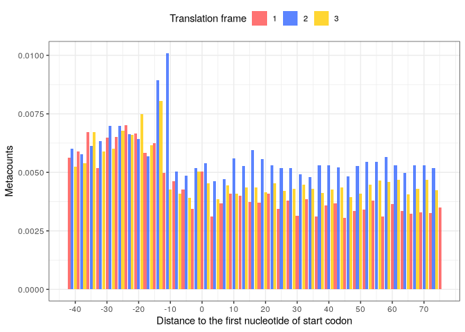
Then, we can visualize the metacounts profile:
plot(start_metacounts)

The user can also specify to group values per translation frame, and also use bars as the position on the profile is a discrete variable: Then, we can visualize the metacounts profile:
p_start_metacounts <- start_metacounts %>%
  plot(from = -42, to = 75,
       translation_frame = TRUE,
       geom = "bar",
       x_lab = "Distance to the first nucleotide of start codon")
p_start_metacounts
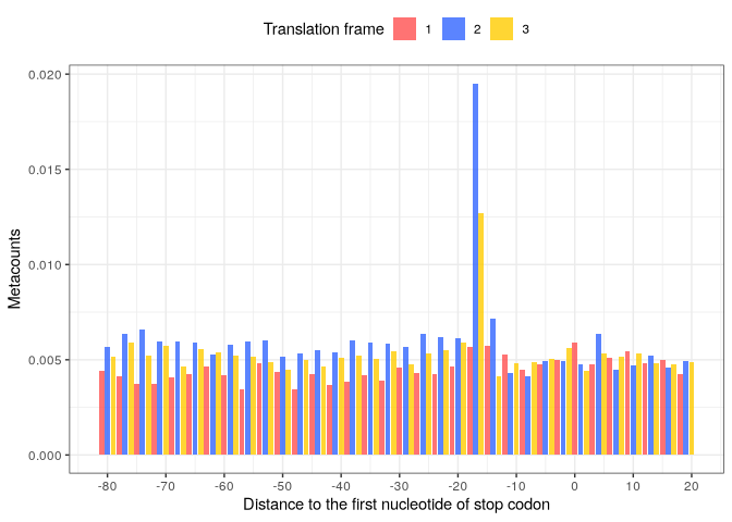
We perform the same for the STOP codon (adjusting for the position of the 1st nucleotide):
stop_tb <- annot %>%
  select(rname=chr, strand, position=end) %>%
  mutate(position = ifelse(strand=='+', position-2, position+2))
stop_metacounts <- metacounts_feature(count_table, stop_tb, width=100)
stop_metacounts %>%
  head(15) %>%
  knitr::kable()
x |
count |
|---|---|
-100 |
0.0055727 |
-99 |
0.0044619 |
-98 |
0.0068743 |
-97 |
0.0061145 |
-96 |
0.0050028 |
-95 |
0.0060474 |
-94 |
0.0051904 |
-93 |
0.0035142 |
-92 |
0.0063497 |
-91 |
0.0061145 |
-90 |
0.0048556 |
-89 |
0.0064173 |
-88 |
0.0056928 |
-87 |
0.0048775 |
-86 |
0.0066952 |
Metacount profile obtained:
stop_metacounts %>%
  plot(from = -81, to = 20,
       translation_frame = TRUE,
       geom = "bar",
       x_lab = "Distance to the first nucleotide of stop codon")
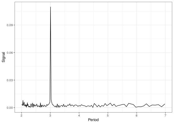
Periodicity
From the genome annotation, we can extract regions corresponding to protein coding genes, compute the metacounts profile for all these regions and use FFT to analyse periodicity in the counts.
cds_tb <- annot %>%
  select(rname = chr, strand, begin=start, end)
fft_tb <- FFT(count_table = count_table,
              region_tb = cds_tb)
fft_tb %>%
  head(15) %>%
  knitr::kable()
signal |
freq |
period |
|---|---|---|
0.1097155 |
137 |
3.007299 |
0.0087828 |
136 |
3.029412 |
0.0079080 |
201 |
2.049751 |
0.0060486 |
197 |
2.091371 |
0.0059655 |
138 |
2.985507 |
0.0056546 |
35 |
11.771429 |
0.0055253 |
57 |
7.228070 |
0.0054040 |
135 |
3.051852 |
0.0053650 |
187 |
2.203209 |
0.0053174 |
53 |
7.773585 |
0.0052531 |
155 |
2.658065 |
0.0052046 |
50 |
8.240000 |
0.0051031 |
32 |
12.875000 |
0.0050365 |
173 |
2.381503 |
0.0049383 |
81 |
5.086420 |
Visualization
p_fft <- fft_tb %>%
  filter(period < 7) %>%
  plot()
p_fft
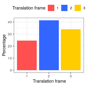
Frame preference
The third analysis provided in this downstream analysis is the count of reads falling into each translation frame (1, 2 or 3). The frame_preference function takes the same inputs as the 2 previous functions.
frame_pref_tb <- frame_preference(count_table = count_table,
                                  region_tb = cds_tb)
frame_pref_tb %>%
  knitr::kable()
frame |
pc |
|---|---|
1 |
24.54694 |
2 |
41.39385 |
3 |
34.05922 |
Visualization
p_frame_pref <- plot(frame_pref_tb)
p_frame_pref
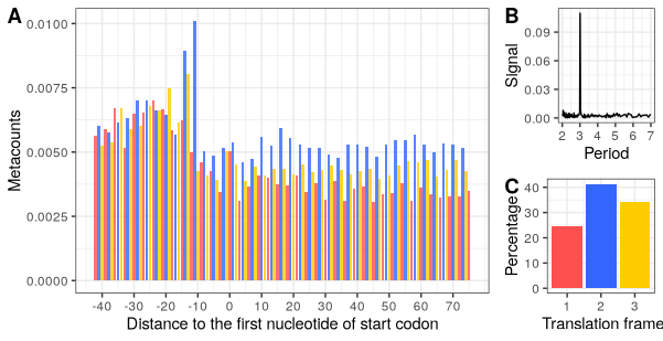
Final plot for the paper:
library(ggpubr)
p1 <- p_start_metacounts + theme(legend.position = "none")
p3 <- p_frame_pref + theme(legend.position = "none")
ggarrange(p1,
          ggarrange(p_fft, p3, nrow=2, labels = c("B","C")),
          widths = c(3,1),
          labels = c("A","")
)
Notebook rendering time and memory:
time_end <- now()
rendering_time <- time_end - time_start
rendering_time
#> Time difference of 20.26483 mins
pryr::mem_used()
#> 1.01 GB