Endonucleolytic cleavage site prediction using 5’-end RNA-Seq data

Complete source of this page is available in the notebook Endoribonucleolytic_sites_prediction.Rmd.

Based on the publication from Broglia L, Lécrivain A-L, Renault TT, Hahnke K, Ahmed-Begrich R, Le Rhun A, Charpentier E (2020) An RNA-seq based comparative approach reveals the transcriptome-wide interplay between 3′-to-5′ exoRNases and RNase Y. Nature Communications, 11, 1587. https://doi.org/10.1038/s41467-020-15387-6

Download datasets

Data from this article are publicly available on the SRA NCBI repository: https://www.ncbi.nlm.nih.gov/sra?term=SRP149896

For this notebook, we will use only 9 RNA-Seq samples corresponding to 9 datasets of Streptococcus pyogenes 5’-end RNA-Seq (SRX4173017, SRX4173016, SRX4173015, SRX4173014, SRX4173013, SRX4173012, SRX4173011, SRX4173010, SRX4173009).

As the datasets are too bug for direct download, fasterq-dump (instead of basic “curl/wget” command) from ncbi/sra-tools must be used to retrieve FASTQ files directly in the extdata directory of the GitLab project in the sub-directory called Spyo_Broglia where the reference genome is already provided when the project is clone:

for i in SRR7269351	SRR7269352 SRR7269353 SRR7269354 SRR7269355 SRR7269356 SRR7269357 SRR7269358 SRR7269359 ; do 
  fasterq-dump $i --outdir ../extdata/Spyo_Broglia ; 
done

We remove all reverse files (rm SRR7236935._2.fastq.gz) and we gzip all forward files.

library(tidyverse)
library(rnaends)

Pre-processing

Thse datasets were already pre-processed when they have been submitted, so we can directly map the FASTQ files on the reference genome.

Quantification

We use the map_fastq_files to map the 9 FASTQ files in a single command.

bf <- map_fastq_files(list_fastq_files = list.files("../extdata/Spyo_Broglia/",
                                                    pattern = ".fastq.gz",
                                                    full.names = TRUE),
                      index_name = "../extdata/Spyo_Broglia/data/spyo_SF370.bt", # Path of the genome index (created if not exists)
                      fasta_name = "../extdata/Spyo_Broglia/spyo_SF370.fasta", # Path of the reference genome file
                      bam_dir = "../extdata/Spyo_Broglia/mapping_results", # Output directory
                      max_map_mismatch = 1,
                      aligner = "bowtie", # Either bowtie or subread
                      map_unique = FALSE,
                      force = F,
                      threads = 3)
#> bam_file '../extdata/Spyo_Broglia/mapping_results/SRR7269351_1.fastq.gz.bam' already exists, set force=TRUE to recompute
#> bam_file '../extdata/Spyo_Broglia/mapping_results/SRR7269352_1.fastq.gz.bam' already exists, set force=TRUE to recompute
#> bam_file '../extdata/Spyo_Broglia/mapping_results/SRR7269353_1.fastq.gz.bam' already exists, set force=TRUE to recompute
#> bam_file '../extdata/Spyo_Broglia/mapping_results/SRR7269354_1.fastq.gz.bam' already exists, set force=TRUE to recompute
#> bam_file '../extdata/Spyo_Broglia/mapping_results/SRR7269355_1.fastq.gz.bam' already exists, set force=TRUE to recompute
#> bam_file '../extdata/Spyo_Broglia/mapping_results/SRR7269356_1.fastq.gz.bam' already exists, set force=TRUE to recompute
#> bam_file '../extdata/Spyo_Broglia/mapping_results/SRR7269357_1.fastq.gz.bam' already exists, set force=TRUE to recompute
#> bam_file '../extdata/Spyo_Broglia/mapping_results/SRR7269358_1.fastq.gz.bam' already exists, set force=TRUE to recompute
#> bam_file '../extdata/Spyo_Broglia/mapping_results/SRR7269359_1.fastq.gz.bam' already exists, set force=TRUE to recompute
bf
#> [[1]]
#> [1] "../extdata/Spyo_Broglia/mapping_results/SRR7269351_1.fastq.gz.bam"
#> 
#> [[2]]
#> [1] "../extdata/Spyo_Broglia/mapping_results/SRR7269352_1.fastq.gz.bam"
#> 
#> [[3]]
#> [1] "../extdata/Spyo_Broglia/mapping_results/SRR7269353_1.fastq.gz.bam"
#> 
#> [[4]]
#> [1] "../extdata/Spyo_Broglia/mapping_results/SRR7269354_1.fastq.gz.bam"
#> 
#> [[5]]
#> [1] "../extdata/Spyo_Broglia/mapping_results/SRR7269355_1.fastq.gz.bam"
#> 
#> [[6]]
#> [1] "../extdata/Spyo_Broglia/mapping_results/SRR7269356_1.fastq.gz.bam"
#> 
#> [[7]]
#> [1] "../extdata/Spyo_Broglia/mapping_results/SRR7269357_1.fastq.gz.bam"
#> 
#> [[8]]
#> [1] "../extdata/Spyo_Broglia/mapping_results/SRR7269358_1.fastq.gz.bam"
#> 
#> [[9]]
#> [1] "../extdata/Spyo_Broglia/mapping_results/SRR7269359_1.fastq.gz.bam"

Mapping statistics

The map_stats_bam_files function provides some basic statistics on the mapping:

map_stats_bam_files(bam_files = bf) %>%
  knitr::kable()
#> BAM file mapping stats exists '../extdata/Spyo_Broglia/mapping_results/SRR7269351_1.fastq.gz.bam.map_stats.csv' already exists, set force=TRUE to recompute
#> BAM file mapping stats exists '../extdata/Spyo_Broglia/mapping_results/SRR7269352_1.fastq.gz.bam.map_stats.csv' already exists, set force=TRUE to recompute
#> BAM file mapping stats exists '../extdata/Spyo_Broglia/mapping_results/SRR7269353_1.fastq.gz.bam.map_stats.csv' already exists, set force=TRUE to recompute
#> BAM file mapping stats exists '../extdata/Spyo_Broglia/mapping_results/SRR7269354_1.fastq.gz.bam.map_stats.csv' already exists, set force=TRUE to recompute
#> BAM file mapping stats exists '../extdata/Spyo_Broglia/mapping_results/SRR7269355_1.fastq.gz.bam.map_stats.csv' already exists, set force=TRUE to recompute
#> BAM file mapping stats exists '../extdata/Spyo_Broglia/mapping_results/SRR7269356_1.fastq.gz.bam.map_stats.csv' already exists, set force=TRUE to recompute
#> BAM file mapping stats exists '../extdata/Spyo_Broglia/mapping_results/SRR7269357_1.fastq.gz.bam.map_stats.csv' already exists, set force=TRUE to recompute
#> BAM file mapping stats exists '../extdata/Spyo_Broglia/mapping_results/SRR7269358_1.fastq.gz.bam.map_stats.csv' already exists, set force=TRUE to recompute
#> BAM file mapping stats exists '../extdata/Spyo_Broglia/mapping_results/SRR7269359_1.fastq.gz.bam.map_stats.csv' already exists, set force=TRUE to recompute

bam_file	mapped	unmapped	pc_mapped
SRR7269351_1.fastq.gz.bam	41814799	988534	97.69
SRR7269352_1.fastq.gz.bam	41739505	938889	97.80
SRR7269353_1.fastq.gz.bam	43357081	1019019	97.70
SRR7269354_1.fastq.gz.bam	43026077	1016127	97.69
SRR7269355_1.fastq.gz.bam	34567930	650684	98.15
SRR7269356_1.fastq.gz.bam	37802063	705215	98.17
SRR7269357_1.fastq.gz.bam	26960617	641089	97.68
SRR7269358_1.fastq.gz.bam	34908063	977130	97.28
SRR7269359_1.fastq.gz.bam	40858741	759768	98.17

Quantification (counts computation)

In order to obtain counts per position, we use the quantify_from_bam_files function to parse previoulsy obtained bam_files.

This function allows the quantification of either the 5’-ends (quantify_5prime) or the 3’-ends (quantify_3prime), in all cases it’s an exact position quantification.

Run with minimal parameters:

count_table <- quantify_from_bam_files(bam_files = bf,
                                       sample_ids = c("WT1", "WT2", "WT3", 
                                                    "Y1", "Y2", "Y3", 
                                                    "suppl1", "suppl2", "suppl3"), # Set an identifier to know the source of each values
                                       fun = quantify_5prime)
#> Quantification 5' output file exists, set force=T to overwrite: ../extdata/Spyo_Broglia/mapping_results/SRR7269351_1.fastq.gz.bam.csv
#> Quantification 5' output file exists, set force=T to overwrite: ../extdata/Spyo_Broglia/mapping_results/SRR7269352_1.fastq.gz.bam.csv
#> Quantification 5' output file exists, set force=T to overwrite: ../extdata/Spyo_Broglia/mapping_results/SRR7269353_1.fastq.gz.bam.csv
#> Quantification 5' output file exists, set force=T to overwrite: ../extdata/Spyo_Broglia/mapping_results/SRR7269354_1.fastq.gz.bam.csv
#> Quantification 5' output file exists, set force=T to overwrite: ../extdata/Spyo_Broglia/mapping_results/SRR7269355_1.fastq.gz.bam.csv
#> Quantification 5' output file exists, set force=T to overwrite: ../extdata/Spyo_Broglia/mapping_results/SRR7269356_1.fastq.gz.bam.csv
#> Quantification 5' output file exists, set force=T to overwrite: ../extdata/Spyo_Broglia/mapping_results/SRR7269357_1.fastq.gz.bam.csv
#> Quantification 5' output file exists, set force=T to overwrite: ../extdata/Spyo_Broglia/mapping_results/SRR7269358_1.fastq.gz.bam.csv
#> Quantification 5' output file exists, set force=T to overwrite: ../extdata/Spyo_Broglia/mapping_results/SRR7269359_1.fastq.gz.bam.csv

count_table %>% 
  head(15) %>%
  knitr::kable()

sample_id	rname	position	strand	count
WT1	AE004092.2	38	+	2
WT1	AE004092.2	205	+	819
WT1	AE004092.2	206	+	13
WT1	AE004092.2	211	+	7
WT1	AE004092.2	215	+	8
WT1	AE004092.2	217	+	34
WT1	AE004092.2	218	+	2
WT1	AE004092.2	219	+	2
WT1	AE004092.2	219	-	5
WT1	AE004092.2	236	+	15
WT1	AE004092.2	248	+	31
WT1	AE004092.2	253	+	13
WT1	AE004092.2	254	+	1
WT1	AE004092.2	262	+	14
WT1	AE004092.2	265	+	117

Downstream analysis

Differential abundances for prediction of cleavage sites

As in the article, we’re going to carry out a differential gene expression analysis (DGE), but at the resolution of an exact position to detect RNase Y endonucleolytic cleavage sites by comparing 3 S. pyogenes strains:

• Wild-type

• RNase Y deletion mutant

• RNAse Y deletion mutant supplemented

To perform a DGE analysis the “edgeR” package is be used (which is not part of the requirements of the rnaends package).

We use as input data the count table we’ve just produced.

library(edgeR)

Pivot the count table to create a DGEList object

group1 <- c("WT", "WT", "WT")
group2 <- c("Y", "Y", "Y")
group3 <- c("suppl", "suppl", "suppl")

# Pivot count table
data <- count_table %>% 
  pivot_wider(id_cols = c(position, strand),
              names_from = sample_id,
              values_from = count, values_fill = 0)

# Transform into matrix for DGElist
mat <- data[,3:ncol(data)] %>% 
  as.matrix()
rownames(mat) <- paste0(data$position, data$strand)
mat %>% 
  head(15) %>%
  knitr::kable()

	WT1	WT2	WT3	Y1	Y2	Y3	suppl1	suppl2	suppl3
38+	2	0	0	0	0	0	0	0	0
205+	819	491	358	1001	345	568	212	304	976
206+	13	22	5	44	17	117	3	4	21
211+	7	11	5	35	0	0	1	1	0
215+	8	1	10	0	4	4	1	0	0
217+	34	13	7	16	2	8	15	1	10
218+	2	0	0	0	0	0	0	0	0
219+	2	0	1	0	0	0	0	0	0
219-	5	0	0	0	0	0	0	0	0
236+	15	0	0	1	0	1	0	0	31
248+	31	15	2	6	0	9	45	0	1
253+	13	0	0	0	0	1	0	0	0
254+	1	0	0	3	0	0	0	0	0
262+	14	0	6	1	3	14	43	0	0
265+	117	33	1	0	15	11	0	0	0

DGEList and filter count according cpm

dge <- DGEList(counts = mat[,1:9], group = factor(c(group1, group2, group3)) )

# Keep position where there is at least 6 conditions with cpm>0.05
keep <- rowSums(cpm(dge) >= 0.05) >= 6
dge.filter <- dge[keep, ]

# Update dge (for racalcul of cpm)
dge2.filter <- DGEList(dge.filter$counts,
                       group = factor(c(group1, group2, group3)) )

# Keep position where there is at least 3 conditions with cpm>5
keep <- rowSums(cpm(dge2.filter) >= 5) >= 3
dge3.filter <- dge2.filter[keep, ] 

cpm(dge3.filter) %>% 
  head(15) %>% knitr::kable()

	WT1	WT2	WT3	Y1	Y2	Y3	suppl1	suppl2	suppl3
205+	22.170898	13.4253747	9.1030977	27.186211	10.908131	16.3304562	8.5810845	9.3700179	26.9990941
2540+	5.820199	2.1054050	7.6028665	1.249316	1.359564	2.5588215	9.9572962	2.3425045	0.2489671
3452+	132.483974	189.8965934	68.4003711	212.057875	77.115743	78.1446831	47.9650241	67.0079572	177.7071523
4499+	6.253330	8.1481908	2.5173371	8.609419	1.960302	1.3225369	3.0357610	1.1712522	0.0276630
4512+	20.790293	7.3825889	7.2977348	14.828842	13.121375	4.6576301	11.6573223	7.3665602	0.1659780
11902+	12.777367	6.4255867	12.4341195	28.082459	14.259615	15.2954273	2.0238407	6.8117565	26.1138779
12203+	10.124439	8.6403634	4.2718447	4.725675	6.797821	6.6414355	1.4571653	7.6131396	0.8852162
13365+	8.418986	3.1991219	4.3481277	5.377492	7.493412	3.7376044	3.3190987	0.7089158	4.5367330
13441+	5.874340	6.9997880	3.6107259	5.784878	2.719128	3.3350932	4.4119727	0.2157570	0.0000000
13446+	12.750297	5.7693565	7.7554324	9.695781	4.584577	8.2514805	24.4075186	1.5719438	0.0276630
13451+	8.121208	0.1093717	9.4590848	7.197149	1.201475	0.5750161	3.4405292	0.3698691	0.2766301
13475+	12.235954	24.9094020	3.1530283	8.745215	4.963990	5.3764002	4.4119727	3.6062240	23.5412183
13527+	1.840807	0.2460863	0.9916782	14.204184	5.469874	6.6126847	0.0404768	0.3082243	21.0792108
13552+	17.541809	6.7263588	0.9662506	8.364988	7.019145	5.4626526	8.0548859	0.4931588	0.0276630
13559+	6.172118	3.8553520	0.3559871	16.376908	1.517653	4.1113649	4.2905422	0.0616449	9.3224331

Normalize and estimate dispersion

Normalization

dge3.filter <- calcNormFactors(dge3.filter, method = "TMM")

Dispersion

disp <- estimateDisp(dge3.filter)
#> Using classic mode.

Exact tests

Comparison WT vs RNase Y deletion mutant

et <- exactTest(disp, pair = c("WT", "Y"))
res_WT <- et$table 
res_WT$fdr <- p.adjust(res_WT$PValue, method = "fdr") # Adjusting p.values
res_WT$Position <- as.integer(str_sub(rownames(res_WT), 1, -2)) # Retrieving positions using stocked into the rownames
res_WT$strand <- str_sub(rownames(res_WT), -1) # Retrieving strand
res_WT %>% 
  head(15) %>%
  knitr::kable()

	logFC	logCPM	PValue	fdr	Position	strand
205+	0.4757538	4.097125	0.6161737	1.0000000	205	+
2540+	-1.2969346	1.768362	0.3370351	1.0000000	2540	+
3452+	0.0168134	6.936504	0.9846036	1.0000000	3452	+
4499+	-0.4542850	1.736353	0.7499819	1.0000000	4499	+
4512+	0.0787080	3.143991	0.9482911	1.0000000	4512	+
11902+	1.0497216	3.917431	0.3388455	1.0000000	11902	+
12203+	-0.0990961	2.468814	0.9318575	1.0000000	12203	+
13365+	0.2956658	2.204602	0.8001578	1.0000000	13365	+
13441+	-0.3248103	1.752619	0.8400716	1.0000000	13441	+
13446+	0.0078938	2.913511	0.9962916	1.0000000	13446	+
13451+	-0.8812748	1.583629	0.5850758	1.0000000	13451	+
13475+	-0.9495031	3.505009	0.4234994	1.0000000	13475	+
13527+	3.3057756	2.826576	0.0722374	0.5765283	13527	+
13552+	-0.0277194	2.451620	0.9866344	1.0000000	13552	+
13559+	1.1973548	2.436253	0.4545305	1.0000000	13559	+

Comparison supplemented RNase Y deletion mutant vs. RNase Y deletion mutant

et <- exactTest(disp, pair = c("suppl", "Y"))
res_suppl <- et$table 
res_suppl$fdr <- p.adjust(res_suppl$PValue, method = "fdr") # Adjusting p.values
res_suppl$Position <- as.integer(str_sub(rownames(res_suppl),1,-2)) # Retrieving positions using stocked into the rownames
res_suppl$strand <- str_sub(rownames(res_suppl),-1) # Retrieving strand
res_suppl %>% 
  head(15) %>%
  knitr::kable()

	logFC	logCPM	PValue	fdr	Position	strand
205+	-0.2700981	4.097125	0.7756757	0.9841472	205	+
2540+	-1.1317669	1.768362	0.4033664	0.8990873	2540	+
3452+	-0.2658754	6.936504	0.7586034	0.9797373	3452	+
4499+	1.4232888	1.736353	0.3289756	0.8528307	4499	+
4512+	0.7377628	3.143991	0.5398056	0.9480726	4512	+
11902+	0.0581356	3.917431	0.9581940	0.9984513	11902	+
12203+	0.7146266	2.468814	0.5326933	0.9457086	12203	+
13365+	0.5319706	2.204602	0.6509544	0.9710619	13365	+
13441+	1.4779476	1.752619	0.3635666	0.8768117	13441	+
13446+	-0.0561098	2.913511	0.9706936	0.9984513	13446	+
13451+	1.0310394	1.583629	0.5285491	0.9456388	13451	+
13475+	-1.3589715	3.505009	0.2557154	0.7890100	13475	+
13527+	-0.5195980	2.826576	0.7595278	0.9799139	13527	+
13552+	1.4159979	2.451620	0.3564504	0.8744636	13552	+
13559+	0.0373990	2.436253	0.9827840	0.9990971	13559	+

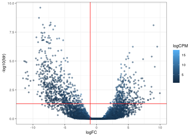
Visualization

res_WT %>% 
  ggplot(aes(x = logFC, y = -log10(fdr), color = logCPM)) +
  geom_point(alpha = 0.5) +
  theme_bw() + 
  geom_vline(xintercept = -1, col = "red") +
  geom_hline(yintercept = -log10(0.05), col = "red")

Merge comparisons and select significant positions

To identify a position as a RNase Y endonucleolytic cleavage site, Broglia et al. keep only positions where the fdr is lower than 0.01 and logFC lower of equal to -1 in both comparison we’ve made.

So we are going to merge our both result tables then filter following these criterias.

res <- res_suppl %>% 
  inner_join(res_WT, by = c("Position","strand"), suffix = c(".suppl", ".WT")) 

Number of cleavage sites identified:

endoY <- res %>% 
  filter(fdr.WT<0.05 & fdr.suppl<0.05 & logFC.WT<= -1 & logFC.suppl<= -1)
endoY %>%
  nrow
#> [1] 532

Number of clusters of cleavage sites identified:

endoY <- endoY %>% 
 arrange(Position) %>%
 mutate(ID = cumsum(c(1, diff(Position) >= 5))) %>% 
 arrange(desc(ID)) 
endoY %>% 
  group_by(ID) %>% 
  n_groups
#> [1] 381

Comparison with Broglia results

We provide a small table of RNase Y cleavage sites identifed by Broglia et al. using 5’-end RNA-Seq in the extdata directory our GitLab project in order to make the comparison.

Number of RNase Y cleavage sites identified using 5’-end RNA-Seq:

csy <- read_csv("../extdata/Spyo_Broglia/RNaseY_cleavage_site_5Prime.csv", show_col_types = F)
csy %>% 
  nrow
#> [1] 190

Number of RNase Y cleavage sites found in common:

common <- endoY %>% 
  inner_join(csy, by="Position")
common %>%
  nrow
#> [1] 119

Number of RNase Y cleavage sites not found by us:

not_found <- csy %>% 
  anti_join(endoY, by ="Position")
not_found %>%
  nrow
#> [1] 71

Number of sites found not significant:

res %>% 
  filter(Position %in% not_found$Position) %>% 
  nrow
#> [1] 32

Number of sites not tested due to CPM filtering:

not_found %>% 
  anti_join(res, by = "Position") %>% 
  nrow 
#> [1] 39