3’-end post-transcriptional modifications exploration and differential proportion analysis
Complete source of this page is available in the notebook Post-transcriptional_modifications.Rmd.
Based on the publication from Xu X, Usher B, Gutierrez C, Barriot R, Arrowsmith TJ, Han X, Redder P, Neyrolles O, Blower TR, Genevaux P (2023) MenT nucleotidyltransferase toxins extend tRNA acceptor stems and can be inhibited by asymmetrical antitoxin binding. Nature Communications, 14, 4644. https://doi.org/10.1038/s41467-023-40264-3.
Download dataset
Data accompanying the article are publicly available on European Nucleotide Archive (ENA) at EBI https://www.ebi.ac.uk/ena/browser/view/PRJEB62085
For this notebook, we will use some RNA-Seq samples multiplexed into one raw FASTQ file to reproduce some results on the action of toxin MenT1 which adds ribonucleotides at the 3’-end of tRNAs as illustrated in figure 3E of the original paper.
The dataset will be directly downloaded in the ../extdata/MenT1 directory of the project (that should be readily available if the GitLab project is cloned).
The initial ../extdata/MenT1 directory contains also the reference sequences of the tRNAs (multifasta file) to which we will align the 3’-end sequencing reads: Msm.reference.tRNAs.with.CCA.fasta.
library(tidyverse)
time_start <- now()
library(rnaends)
options(width = 250)

data_dir <- "../extdata/MenT1"

raw_fastq <- paste0(data_dir, "/Msm.total.RNA.MenT1.Library.fq.gz")

if (!file.exists(raw_fastq))
    download.file("ftp://ftp.sra.ebi.ac.uk/vol1/run/ERR114/ERR11439143/Msm.total.RNA.MenT1.Library.fq.gz",
                  destfile = raw_fastq)
Pre-processing of reads prior mapping
In this section, we will parse the raw reads to:
validate their content
split the FASTQ file into 4 different FASTQ files, each one of them corresponding to a sample: control without toxin or tRNAs with toxin and replicate 1 or 2
For more information on the other pre-processing features available, see the vignette on pre-processing features.
The reads are 100 nt long and their structure can be schematized as follows:
read position: 1   2                      6                      25    40                 46
               N · multiplexing barcode · recognition sequence · UMI · control sequence · 3'-5' tRNA-end reverse complement
               │   │                      │                       │       │               └ 55nt long
               │   │                      │                       │       └ must be AGATAC
               │   │                      │                       └ 15 random nucleotides (A, T, C or G) serving as
               │   │                      │                         Unique Molecule Identifier (UMI) for PCR duplicates removal
               │   │                      └ must be CGGCACCAACCGAGGCTCA
               │   └ must be one of ACAC, ATTG, GACG or GGTA
               │
               └ one random nucleotide at the beginning
Here, we define the authorized barcodes and their associated experimental condition (in same order) so that we can reuse them later.
barcodes   <- c("ACAC",    "ATTG",    "GACG",     "GGTA")
conditions <- c("ctrl.r1", "ctrl.r2", "MenT1.r1", "MenT1.r2")
The above schematized structure is translated to a read_features table that will be used for reads parsing and validation.
For its initialization, the user must specify which region on the reads contains the sequence destined to be aligned on the reference sequences.
read_features <- init_read_features(start = 46, width = 55) # region to map
read_features %>%
  knitr::kable()
name |
start |
width |
pattern_type |
pattern |
max_mismatch |
readid_prepend |
|---|---|---|---|---|---|---|
readseq |
46 |
55 |
nucleotides |
ACTG |
0 |
FALSE |
Then, the table is updated with each structure element of the reads.
The barcode from position 2 to 5 is a feature of type “constant” which is a set of authorized constant string at a certain location:
read_features <- add_read_feature(read_features,
                                  name = "barcode",
                                  start = 2,
                                  width = 4,
                                  pattern = barcodes,
                                  pattern_type = "constant")
The UMI from position 25 to 39 are composed of A, T, C or G, thus is a feature of type “nucleotides” which is a string composed of a certain alphabet. This feature will be extracted and stored in the read identifier for future use in the quantification step (to remove PCR duplicates), thus the readid_prepend = TRUE argument).
read_features <- add_read_feature(read_features,
                                  name = "UMI",
                                  start = 25,
                                  width = 15,
                                  pattern = "ACGT",
                                  pattern_type =  "nucleotides",
                                  readid_prepend = TRUE)
Then, the recognition sequence and the control sequence correspond to constant character strings and will be used to validate the reads. These are features of type “constant”.
read_features <- add_read_feature(read_features,
                                  name = "recognition_seq",
                                  start = 6,
                                  width = 19,
                                  pattern = "CGGCACCAACCGAGGCTCA",
                                  pattern_type = "constant",
                                  max_mismatch = 1,
                                  readid_prepend = FALSE)
read_features <- add_read_feature(read_features,
                                  name = "control_seq",
                                  start = 40,
                                  width = 6,
                                  pattern = "AGATAC",
                                  pattern_type = "constant",
                                  readid_prepend = FALSE)
read_features %>%
  knitr::kable()
name |
start |
width |
pattern_type |
pattern |
max_mismatch |
readid_prepend |
|---|---|---|---|---|---|---|
readseq |
46 |
55 |
nucleotides |
ACTG |
0 |
FALSE |
barcode |
2 |
4 |
constant |
ACAC, AT…. |
0 |
FALSE |
UMI |
25 |
15 |
nucleotides |
ACGT |
0 |
TRUE |
recognition_seq |
6 |
19 |
constant |
CGGCACCA…. |
1 |
FALSE |
control_seq |
40 |
6 |
constant |
AGATAC |
0 |
FALSE |
Once the read_featurestable is defined, parsing of read can be performed. As we need also to demultiplex the samples here, we will directly calldemultiplexwhich will call theparse_read` internally to parse and validate the reads.
Demultiplex original raw FASTQ file(s) into separate FASTQ files
Reads are validated against the read features and only valid reads are found in the demultiplexed FASTQ files.
demux_report <- demultiplex(fastq_file = raw_fastq,
                            yieldsize = 1e6, # number of reads parsed at each iteration
                            features = read_features,
                            force = TRUE, # demultiplex will not do anything if there already exists a report
                            keep_invalid_reads = FALSE) # FALSE: we do not want invalid reads to be returned in a separate FASTQ file
demux_report %>%
  knitr::kable()
barcode_group |
is_valid_readseq |
is_valid_barcode |
is_valid_UMI |
is_valid_recognition_seq |
is_valid_control_seq |
count |
demux_filename |
|---|---|---|---|---|---|---|---|
ACAC |
FALSE |
TRUE |
TRUE |
TRUE |
TRUE |
39 |
NA |
ACAC |
TRUE |
TRUE |
TRUE |
TRUE |
TRUE |
996140 |
../extdata/MenT1/Msm.total.RNA.MenT1.Library_demux/Msm.total.RNA.MenT1.Library_ACAC_valid.fastq.gz |
ATTG |
FALSE |
TRUE |
TRUE |
TRUE |
TRUE |
35 |
NA |
ATTG |
TRUE |
TRUE |
TRUE |
TRUE |
TRUE |
761196 |
../extdata/MenT1/Msm.total.RNA.MenT1.Library_demux/Msm.total.RNA.MenT1.Library_ATTG_valid.fastq.gz |
GACG |
FALSE |
TRUE |
TRUE |
TRUE |
TRUE |
25 |
NA |
GACG |
TRUE |
TRUE |
TRUE |
TRUE |
TRUE |
614477 |
../extdata/MenT1/Msm.total.RNA.MenT1.Library_demux/Msm.total.RNA.MenT1.Library_GACG_valid.fastq.gz |
GGTA |
FALSE |
TRUE |
TRUE |
TRUE |
TRUE |
39 |
NA |
GGTA |
TRUE |
TRUE |
TRUE |
TRUE |
TRUE |
1059530 |
../extdata/MenT1/Msm.total.RNA.MenT1.Library_demux/Msm.total.RNA.MenT1.Library_GGTA_valid.fastq.gz |
The report provides statistics on reads for each sample together with the fastq output file.
Mapping of reads and quantification of 3’-ends abundances in a count table
As, reads should align partially, we will use subread.
# input
demux_dir <- paste0(sub("(.fastq|.fq)(.gz)?$", "", raw_fastq), "_demux")
fastq_files <- demux_report$demux_filename %>%
na.omit()
# params for mapping
reference_genome <- "Msm.reference.tRNAs.with.CCA.fasta"
reference_fasta <- paste0(data_dir, "/", reference_genome)
reference_index <- paste0(data_dir, "/", reference_genome, ".subread")
aligner <- "subread"
max_mismatch <- 0
bam_dir <- paste0(demux_dir,
"/mm",
max_mismatch,
"_",
aligner,
"_",
reference_genome)
# perform mapping
bam_files <- lapply(
fastq_files,
map_fastq,
fasta_name = reference_fasta,
index_name = reference_index,
max_map_mismatch = max_mismatch,
aligner = aligner,
force = TRUE,
bam_dir = bam_dir,
threads = 4
)
#> [1] "Index directory already exists remove it if you want to recreate it"
#>
#> ========== _____ _ _ ____ _____ ______ _____
#> ===== / ____| | | | _ \| __ \| ____| /\ | __ \
#> ===== | (___ | | | | |_) | |__) | |__ / \ | | | |
#> ==== \___ \| | | | _ <| _ /| __| / /\ \ | | | |
#> ==== ____) | |__| | |_) | | \ \| |____ / ____ \| |__| |
#> ========== |_____/ \____/|____/|_| \_\______/_/ \_\_____/
#> Rsubread 2.20.0
#>
#> //================================= setting ==================================\\
#> || ||
#> || Function : Read alignment (DNA-Seq) ||
#> || Input file : Msm.total.RNA.MenT1.Library_ACAC_valid.fastq.gz ||
#> || Output file : Msm.total.RNA.MenT1.Library_ACAC_valid.fastq.gz.bam (B ... ||
#> || Index name : index ||
#> || ||
#> || ------------------------------------ ||
#> || ||
#> || Threads : 4 ||
#> || Phred offset : 33 ||
#> || Min votes : 3 / 10 ||
#> || Max mismatches : 0 ||
#> || Max indel length : 0 ||
#> || Report multi-mapping reads : no ||
#> || Max alignments per multi-mapping read : 1 ||
#> || ||
#> \\============================================================================//
#>
#> //================ Running (02-Nov-2025 20:39:31, pid=540209) ================\\
#> || ||
#> || Check the input reads. ||
#> || The input file contains base space reads. ||
#> || Initialise the memory objects. ||
#> || Estimate the mean read length. ||
#> || The range of Phred scores observed in the data is [3,39] ||
#> || Create the output BAM file. ||
#> || Check the index. ||
#> || Init the voting space. ||
#> || Global environment is initialised. ||
#> || Load the 1-th index block... ||
#> || The index block has been loaded. ||
#> || Start read mapping in chunk. ||
#> || 2% completed, 0.3 mins elapsed, rate=568.4k reads per second ||
#> || 9% completed, 0.3 mins elapsed, rate=652.5k reads per second ||
#> || 16% completed, 0.3 mins elapsed, rate=667.8k reads per second ||
#> || 23% completed, 0.3 mins elapsed, rate=674.6k reads per second ||
#> || 29% completed, 0.3 mins elapsed, rate=679.7k reads per second ||
#> || 36% completed, 0.3 mins elapsed, rate=682.4k reads per second ||
#> || 42% completed, 0.3 mins elapsed, rate=683.3k reads per second ||
#> || 49% completed, 0.3 mins elapsed, rate=684.3k reads per second ||
#> || 56% completed, 0.3 mins elapsed, rate=685.4k reads per second ||
#> || 63% completed, 0.3 mins elapsed, rate=685.4k reads per second ||
#> || 70% completed, 0.3 mins elapsed, rate=34.4k reads per second ||
#> || 73% completed, 0.3 mins elapsed, rate=35.8k reads per second ||
#> || 76% completed, 0.3 mins elapsed, rate=37.3k reads per second ||
#> || 79% completed, 0.3 mins elapsed, rate=38.7k reads per second ||
#> || 83% completed, 0.3 mins elapsed, rate=40.1k reads per second ||
#> || 86% completed, 0.3 mins elapsed, rate=41.5k reads per second ||
#> || 89% completed, 0.3 mins elapsed, rate=42.9k reads per second ||
#> || 93% completed, 0.4 mins elapsed, rate=44.6k reads per second ||
#> || 97% completed, 0.4 mins elapsed, rate=45.9k reads per second ||
#> || ||
#> || Completed successfully. ||
#> || ||
#> \\==================================== ====================================//
#>
#> //================================ Summary =================================\\
#> || ||
#> || Total reads : 996,140 ||
#> || Mapped : 688,081 (69.1%) ||
#> || Uniquely mapped : 688,081 ||
#> || Multi-mapping : 0 ||
#> || ||
#> || Unmapped : 308,059 ||
#> || ||
#> || Indels : 0 ||
#> || ||
#> || Running time : 0.4 minutes ||
#> || ||
#> \\============================================================================//
#>
#> [1] "Index directory already exists remove it if you want to recreate it"
#>
#> ========== _____ _ _ ____ _____ ______ _____
#> ===== / ____| | | | _ \| __ \| ____| /\ | __ \
#> ===== | (___ | | | | |_) | |__) | |__ / \ | | | |
#> ==== \___ \| | | | _ <| _ /| __| / /\ \ | | | |
#> ==== ____) | |__| | |_) | | \ \| |____ / ____ \| |__| |
#> ========== |_____/ \____/|____/|_| \_\______/_/ \_\_____/
#> Rsubread 2.20.0
#>
#> //================================= setting ==================================\\
#> || ||
#> || Function : Read alignment (DNA-Seq) ||
#> || Input file : Msm.total.RNA.MenT1.Library_ATTG_valid.fastq.gz ||
#> || Output file : Msm.total.RNA.MenT1.Library_ATTG_valid.fastq.gz.bam (B ... ||
#> || Index name : index ||
#> || ||
#> || ------------------------------------ ||
#> || ||
#> || Threads : 4 ||
#> || Phred offset : 33 ||
#> || Min votes : 3 / 10 ||
#> || Max mismatches : 0 ||
#> || Max indel length : 0 ||
#> || Report multi-mapping reads : no ||
#> || Max alignments per multi-mapping read : 1 ||
#> || ||
#> \\============================================================================//
#>
#> //================ Running (02-Nov-2025 20:39:53, pid=540209) ================\\
#> || ||
#> || Check the input reads. ||
#> || The input file contains base space reads. ||
#> || Initialise the memory objects. ||
#> || Estimate the mean read length. ||
#> || The range of Phred scores observed in the data is [3,39] ||
#> || Create the output BAM file. ||
#> || Check the index. ||
#> || Init the voting space. ||
#> || Global environment is initialised. ||
#> || Load the 1-th index block... ||
#> || The index block has been loaded. ||
#> || Start read mapping in chunk. ||
#> || 3% completed, 0.3 mins elapsed, rate=631.3k reads per second ||
#> || 10% completed, 0.3 mins elapsed, rate=657.8k reads per second ||
#> || 17% completed, 0.3 mins elapsed, rate=670.0k reads per second ||
#> || 24% completed, 0.3 mins elapsed, rate=674.9k reads per second ||
#> || 31% completed, 0.3 mins elapsed, rate=674.4k reads per second ||
#> || 38% completed, 0.3 mins elapsed, rate=674.7k reads per second ||
#> || 44% completed, 0.3 mins elapsed, rate=674.6k reads per second ||
#> || 51% completed, 0.3 mins elapsed, rate=674.9k reads per second ||
#> || 58% completed, 0.3 mins elapsed, rate=675.4k reads per second ||
#> || 65% completed, 0.3 mins elapsed, rate=675.5k reads per second ||
#> || 69% completed, 0.3 mins elapsed, rate=26.7k reads per second ||
#> || 73% completed, 0.3 mins elapsed, rate=27.9k reads per second ||
#> || 76% completed, 0.3 mins elapsed, rate=29.0k reads per second ||
#> || 79% completed, 0.3 mins elapsed, rate=30.2k reads per second ||
#> || 82% completed, 0.3 mins elapsed, rate=31.3k reads per second ||
#> || 86% completed, 0.3 mins elapsed, rate=32.4k reads per second ||
#> || 89% completed, 0.3 mins elapsed, rate=33.5k reads per second ||
#> || 92% completed, 0.3 mins elapsed, rate=34.6k reads per second ||
#> || 96% completed, 0.3 mins elapsed, rate=35.8k reads per second ||
#> || 99% completed, 0.3 mins elapsed, rate=36.9k reads per second ||
#> || ||
#> || Completed successfully. ||
#> || ||
#> \\==================================== ====================================//
#>
#> //================================ Summary =================================\\
#> || ||
#> || Total reads : 761,196 ||
#> || Mapped : 456,291 (59.9%) ||
#> || Uniquely mapped : 456,291 ||
#> || Multi-mapping : 0 ||
#> || ||
#> || Unmapped : 304,905 ||
#> || ||
#> || Indels : 0 ||
#> || ||
#> || Running time : 0.4 minutes ||
#> || ||
#> \\============================================================================//
#>
#> [1] "Index directory already exists remove it if you want to recreate it"
#>
#> ========== _____ _ _ ____ _____ ______ _____
#> ===== / ____| | | | _ \| __ \| ____| /\ | __ \
#> ===== | (___ | | | | |_) | |__) | |__ / \ | | | |
#> ==== \___ \| | | | _ <| _ /| __| / /\ \ | | | |
#> ==== ____) | |__| | |_) | | \ \| |____ / ____ \| |__| |
#> ========== |_____/ \____/|____/|_| \_\______/_/ \_\_____/
#> Rsubread 2.20.0
#>
#> //================================= setting ==================================\\
#> || ||
#> || Function : Read alignment (DNA-Seq) ||
#> || Input file : Msm.total.RNA.MenT1.Library_GACG_valid.fastq.gz ||
#> || Output file : Msm.total.RNA.MenT1.Library_GACG_valid.fastq.gz.bam (B ... ||
#> || Index name : index ||
#> || ||
#> || ------------------------------------ ||
#> || ||
#> || Threads : 4 ||
#> || Phred offset : 33 ||
#> || Min votes : 3 / 10 ||
#> || Max mismatches : 0 ||
#> || Max indel length : 0 ||
#> || Report multi-mapping reads : no ||
#> || Max alignments per multi-mapping read : 1 ||
#> || ||
#> \\============================================================================//
#>
#> //================ Running (02-Nov-2025 20:40:14, pid=540209) ================\\
#> || ||
#> || Check the input reads. ||
#> || The input file contains base space reads. ||
#> || Initialise the memory objects. ||
#> || Estimate the mean read length. ||
#> || The range of Phred scores observed in the data is [3,39] ||
#> || Create the output BAM file. ||
#> || Check the index. ||
#> || Init the voting space. ||
#> || Global environment is initialised. ||
#> || Load the 1-th index block... ||
#> || The index block has been loaded. ||
#> || Start read mapping in chunk. ||
#> || 3% completed, 0.3 mins elapsed, rate=598.9k reads per second ||
#> || 10% completed, 0.3 mins elapsed, rate=643.9k reads per second ||
#> || 17% completed, 0.3 mins elapsed, rate=659.1k reads per second ||
#> || 24% completed, 0.3 mins elapsed, rate=665.5k reads per second ||
#> || 31% completed, 0.3 mins elapsed, rate=669.2k reads per second ||
#> || 37% completed, 0.3 mins elapsed, rate=671.2k reads per second ||
#> || 44% completed, 0.3 mins elapsed, rate=672.2k reads per second ||
#> || 51% completed, 0.3 mins elapsed, rate=672.7k reads per second ||
#> || 58% completed, 0.3 mins elapsed, rate=673.7k reads per second ||
#> || 65% completed, 0.3 mins elapsed, rate=674.0k reads per second ||
#> || 70% completed, 0.3 mins elapsed, rate=21.8k reads per second ||
#> || 73% completed, 0.3 mins elapsed, rate=22.7k reads per second ||
#> || 76% completed, 0.3 mins elapsed, rate=23.7k reads per second ||
#> || 80% completed, 0.3 mins elapsed, rate=24.7k reads per second ||
#> || 83% completed, 0.3 mins elapsed, rate=25.6k reads per second ||
#> || 86% completed, 0.3 mins elapsed, rate=26.5k reads per second ||
#> || 90% completed, 0.3 mins elapsed, rate=27.5k reads per second ||
#> || 93% completed, 0.3 mins elapsed, rate=28.5k reads per second ||
#> || 97% completed, 0.3 mins elapsed, rate=29.4k reads per second ||
#> || ||
#> || Completed successfully. ||
#> || ||
#> \\==================================== ====================================//
#>
#> //================================ Summary =================================\\
#> || ||
#> || Total reads : 614,477 ||
#> || Mapped : 336,372 (54.7%) ||
#> || Uniquely mapped : 336,372 ||
#> || Multi-mapping : 0 ||
#> || ||
#> || Unmapped : 278,105 ||
#> || ||
#> || Indels : 0 ||
#> || ||
#> || Running time : 0.3 minutes ||
#> || ||
#> \\============================================================================//
#>
#> [1] "Index directory already exists remove it if you want to recreate it"
#>
#> ========== _____ _ _ ____ _____ ______ _____
#> ===== / ____| | | | _ \| __ \| ____| /\ | __ \
#> ===== | (___ | | | | |_) | |__) | |__ / \ | | | |
#> ==== \___ \| | | | _ <| _ /| __| / /\ \ | | | |
#> ==== ____) | |__| | |_) | | \ \| |____ / ____ \| |__| |
#> ========== |_____/ \____/|____/|_| \_\______/_/ \_\_____/
#> Rsubread 2.20.0
#>
#> //================================= setting ==================================\\
#> || ||
#> || Function : Read alignment (DNA-Seq) ||
#> || Input file : Msm.total.RNA.MenT1.Library_GGTA_valid.fastq.gz ||
#> || Output file : Msm.total.RNA.MenT1.Library_GGTA_valid.fastq.gz.bam (B ... ||
#> || Index name : index ||
#> || ||
#> || ------------------------------------ ||
#> || ||
#> || Threads : 4 ||
#> || Phred offset : 33 ||
#> || Min votes : 3 / 10 ||
#> || Max mismatches : 0 ||
#> || Max indel length : 0 ||
#> || Report multi-mapping reads : no ||
#> || Max alignments per multi-mapping read : 1 ||
#> || ||
#> \\============================================================================//
#>
#> //================ Running (02-Nov-2025 20:40:35, pid=540209) ================\\
#> || ||
#> || Check the input reads. ||
#> || The input file contains base space reads. ||
#> || Initialise the memory objects. ||
#> || Estimate the mean read length. ||
#> || The range of Phred scores observed in the data is [3,39] ||
#> || Create the output BAM file. ||
#> || Check the index. ||
#> || Init the voting space. ||
#> || Global environment is initialised. ||
#> || Load the 1-th index block... ||
#> || The index block has been loaded. ||
#> || Start read mapping in chunk. ||
#> || 2% completed, 0.3 mins elapsed, rate=608.6k reads per second ||
#> || 8% completed, 0.3 mins elapsed, rate=658.1k reads per second ||
#> || 15% completed, 0.3 mins elapsed, rate=667.4k reads per second ||
#> || 22% completed, 0.3 mins elapsed, rate=670.3k reads per second ||
#> || 29% completed, 0.3 mins elapsed, rate=671.4k reads per second ||
#> || 36% completed, 0.3 mins elapsed, rate=672.3k reads per second ||
#> || 42% completed, 0.3 mins elapsed, rate=673.0k reads per second ||
#> || 49% completed, 0.3 mins elapsed, rate=672.8k reads per second ||
#> || 56% completed, 0.3 mins elapsed, rate=673.0k reads per second ||
#> || 63% completed, 0.3 mins elapsed, rate=672.5k reads per second ||
#> || 70% completed, 0.3 mins elapsed, rate=36.0k reads per second ||
#> || 73% completed, 0.3 mins elapsed, rate=37.6k reads per second ||
#> || 76% completed, 0.3 mins elapsed, rate=39.1k reads per second ||
#> || 80% completed, 0.3 mins elapsed, rate=40.6k reads per second ||
#> || 83% completed, 0.4 mins elapsed, rate=42.2k reads per second ||
#> || 86% completed, 0.4 mins elapsed, rate=43.6k reads per second ||
#> || 90% completed, 0.4 mins elapsed, rate=45.2k reads per second ||
#> || 94% completed, 0.4 mins elapsed, rate=46.7k reads per second ||
#> || 97% completed, 0.4 mins elapsed, rate=48.2k reads per second ||
#> || ||
#> || Completed successfully. ||
#> || ||
#> \\==================================== ====================================//
#>
#> //================================ Summary =================================\\
#> || ||
#> || Total reads : 1,059,530 ||
#> || Mapped : 754,701 (71.2%) ||
#> || Uniquely mapped : 754,701 ||
#> || Multi-mapping : 0 ||
#> || ||
#> || Unmapped : 304,829 ||
#> || ||
#> || Indels : 0 ||
#> || ||
#> || Running time : 0.4 minutes ||
#> || ||
#> \\============================================================================//
Convert bam files to count table with quantify_3prime
The quantify_3prime is called on each BAM file. The features table is passed to take into account the UMIs that were present in the reads to remove duplicates.
count_table <- quantify_from_bam_files(bam_files,
                                       conditions,
                                       quantify_3prime,
                                       features = read_features,
                                       min_mapped_length = 20,
                                       rev_comp_reads = TRUE,
                                       keep_UMI = FALSE,
                                       force = TRUE)
count_table %>%
  head(15) %>%
  knitr::kable()
sample_id |
rname |
position |
strand |
downstream_seq |
reads |
count |
|---|---|---|---|---|---|---|
ctrl.r1 |
Msm.Ala-CGC.trna33 |
25 |
+ |
ACCACACAG |
1 |
1 |
ctrl.r1 |
Msm.Ala-CGC.trna33 |
25 |
+ |
ACCACACAGGCAGTGTGGGGGCCAGG |
1 |
1 |
ctrl.r1 |
Msm.Ala-CGC.trna33 |
25 |
+ |
ACCACACAGGCAGTGTGGGGGT |
1 |
1 |
ctrl.r1 |
Msm.Ala-CGC.trna33 |
25 |
+ |
ACCACACGGGCAGT |
1 |
1 |
ctrl.r1 |
Msm.Ala-CGC.trna33 |
25 |
+ |
ACCACACGGGCAGTGTGGGGGCCAGGGGTTA |
1 |
1 |
ctrl.r1 |
Msm.Ala-CGC.trna33 |
25 |
+ |
ACCACACGGGCAGTGTGGGGGTCAGG |
1 |
1 |
ctrl.r1 |
Msm.Ala-CGC.trna33 |
25 |
+ |
ACCACACGGGCAGTGTGGGGGTTAGG |
1 |
1 |
ctrl.r1 |
Msm.Ala-CGC.trna33 |
25 |
+ |
ACCACACTGGGAGT |
1 |
1 |
ctrl.r1 |
Msm.Ala-CGC.trna33 |
25 |
+ |
ACCACACTGGTAG |
1 |
1 |
ctrl.r1 |
Msm.Ala-CGC.trna33 |
25 |
+ |
ACCACACTGGTAGT |
1 |
1 |
ctrl.r1 |
Msm.Ala-CGC.trna33 |
25 |
+ |
ACCACACTGGTAGTGTGGGGGTCAGGG |
1 |
1 |
ctrl.r1 |
Msm.Ala-CGC.trna33 |
25 |
+ |
ACCACACTGTCTCCTAGGCTCCACCA |
1 |
1 |
ctrl.r1 |
Msm.Ala-CGC.trna33 |
25 |
+ |
ACCACACTTGCAGTGTGTGGGTCAGGG |
1 |
1 |
ctrl.r1 |
Msm.Ala-CGC.trna33 |
25 |
+ |
ACCACAGTGCTGCACGGCGGTCTGATC |
1 |
1 |
ctrl.r1 |
Msm.Ala-CGC.trna33 |
25 |
+ |
ACCACAGTGGCAGT |
1 |
1 |
Downstream analysis: 3’-end post-transciptional modifications exploration
Pivot count_table to have counts for each sample for the same 3’-end. For noise reduction, we will only keep rows for which there are at least 10 reads in one sample.
count_table_w <- count_table %>%
  select(-reads) %>%
  pivot_wider(names_from = "sample_id", values_from = "count", values_fill = 0) %>%
  filter(if_any(all_of(conditions), ~ . >= 10))
count_table_w %>%
  head(15) %>%
  knitr::kable()
rname |
position |
strand |
downstream_seq |
ctrl.r1 |
ctrl.r2 |
MenT1.r1 |
MenT1.r2 |
|---|---|---|---|---|---|---|---|
Msm.Ala-CGC.trna33 |
26 |
+ |
137 |
2 |
6 |
145 |
|
Msm.Ala-CGC.trna33 |
27 |
+ |
130 |
12 |
15 |
151 |
|
Msm.Ala-CGC.trna33 |
28 |
+ |
79 |
5 |
12 |
86 |
|
Msm.Ala-CGC.trna33 |
29 |
+ |
75 |
12 |
15 |
93 |
|
Msm.Ala-CGC.trna33 |
30 |
+ |
58 |
27 |
25 |
78 |
|
Msm.Ala-CGC.trna33 |
31 |
+ |
62 |
5 |
8 |
78 |
|
Msm.Ala-CGC.trna33 |
32 |
+ |
36 |
5 |
5 |
41 |
|
Msm.Ala-CGC.trna33 |
33 |
+ |
72 |
31 |
29 |
91 |
|
Msm.Ala-CGC.trna33 |
34 |
+ |
72 |
99 |
106 |
99 |
|
Msm.Ala-CGC.trna33 |
35 |
+ |
142 |
341 |
382 |
166 |
|
Msm.Ala-CGC.trna33 |
36 |
+ |
167 |
44 |
55 |
150 |
|
Msm.Ala-CGC.trna33 |
37 |
+ |
158 |
107 |
95 |
115 |
|
Msm.Ala-CGC.trna33 |
38 |
+ |
66 |
13 |
8 |
59 |
|
Msm.Ala-CGC.trna33 |
39 |
+ |
113 |
18 |
20 |
106 |
|
Msm.Ala-CGC.trna33 |
40 |
+ |
146 |
8 |
6 |
132 |
Next, we are going to focus on full length tRNAs. Thus, we will need their length.
tRNAs with expected length from reference sequences FASTA file:
library(Biostrings)
tRNAs_DNASS <- readDNAStringSet(paste0(data_dir, "/", reference_genome))
tRNAs <- tibble(rlength = width(tRNAs_DNASS),
                seq = as.character(tRNAs_DNASS),
                name = names(tRNAs_DNASS)) %>%
  mutate(id = str_extract(name, "trna\\d+.\\S+"),
         rname = as.factor(str_extract(name, "^\\S+"))) %>%
  select(rname, rlength, seq)
tRNAs %>%
  head(15) %>%
  knitr::kable()
rname |
rlength |
seq |
|---|---|---|
Msm.Ala-CGC.trna33 |
76 |
GGGGCTATGGCGCAGTTGGTAGCGCGACTCGTTCGCATCGAGTAGGTCAGGGGTTCGATTCCCCTTAGCTCCACCA |
Msm.Ala-GGC.trna9 |
76 |
GGGGCTATGGCGCAGTTGGTAGCGCACCACACTGGCAGTGTGGGGGTCAGGGGTTCGAATCCCCTTAGCTCCACCA |
Msm.Ala-TGC.trna2 |
76 |
GGGGCCTTAGCTCAGTTGGTAGAGCGCTGCCTTTGCAAGGCAGATGTCAGGAGTTCGAATCTCCTAGGCTCCACCA |
Msm.Arg-ACG.trna27 |
76 |
GCGCCCGTAGCTCAACGGATAGAGCATCTGACTACGGATCAGAAGGTTAGGGGTTCGAATCCCTTCGGGCGCACCA |
Msm.Arg-TCT.trna15 |
76 |
GCCTCCGTAGCTCAATGGATAGAGCATCGGCCTTCTAATCCGACGGTTGCAGGTTCGAGTCCTGCCGGGGGCGCCA |
Msm.Arg-CCG.trna18 |
76 |
GCCCCCGTAGCTCAGGGGATAGAGCGTCTGCCTCCGGAGCAGAAGGCCGCAGGTTCGAATCCTGCCGGGGGCACCA |
Msm.Arg-CCT.trna20 |
76 |
GCCCTCGTAGCTCAGGGGATAGAGCACGGCTCTCCTAAAGCCGGTGTCGCAGGTTCGAATCCTGCCGGGGGCACCA |
Msm.Asn-GTT.trna37 |
76 |
TCCCCTGTAGCTCAATTGGCAGAGCATTCGGCTGTTAACCGAAGGGTTGCTGGTTCGAGTCCAGCCGGGGGAGCCA |
Msm.Asp-GTC.trna31 |
77 |
GGCCCTGTGGCGCAGTTGGTTAGCGCGCCGCCCTGTCACGGCGGAGGTCGCGGGTTCAAGTCCCGTCAGGGTCGCCA |
Msm.Cys-GCA.trna40 |
74 |
GCGGGTGTGGCTGAGTGGCTAGGCAGCGGCCTGCAAAGCCGTCTACACGGGTTCGAGTCCCGTCACTCGCTCCA |
Msm.Cys-GCA.trna44 |
74 |
GGTGGAGTGGCCGAGTGGTGAGGCAACGGCCTGCAAAGCCGTGCACACGGGTTCGATTCCCGTCTCCACCTCCA |
Msm.Gln-CTG.trna10 |
75 |
TGGGGTATGGTGTAATTGGCAACACAGCTGATTCTGGTTCAGCCATTCTAGGTTCGAGTCCTGGTACCCCAGCCA |
Msm.Gln-TTG.trna19 |
75 |
TCCGTCGTGGTGTAATCGGCAGCACCTCTGATTTTGGTTCAGATAGTTCAGGTTCGAGTCCTGGCGACGGAGCCA |
Msm.Glu-CTC.trna11 |
76 |
GCCCCCGTCGTCTAGCGGCCTAGGACGCCGCCCTCTCACGGCGGTAGCGTGGGTTCGAATCCCATCGGGGGTACCA |
Msm.Glu-TTC.trna30 |
76 |
GCCCCCATCGTCTAGTGGCCTAGGACGCCGCCCTTTCACGGCGGTAGCACGGGTTCGAATCCCGTTGGGGGTACCA |
Filter only full length tRNAs with or without Cs added post-transcriptionaly
count_table_w <- tRNAs %>%
  select(-seq) %>%
  inner_join(count_table_w, by = join_by(rname)) %>%
  filter(position == rlength, str_detect(downstream_seq, pattern = "^C*$"))
count_table_w %>%
  knitr::kable()
rname |
rlength |
position |
strand |
downstream_seq |
ctrl.r1 |
ctrl.r2 |
MenT1.r1 |
MenT1.r2 |
|---|---|---|---|---|---|---|---|---|
Msm.Ala-CGC.trna33 |
76 |
76 |
+ |
74878 |
35268 |
14950 |
49270 |
|
Msm.Ala-CGC.trna33 |
76 |
76 |
+ |
C |
48 |
6 |
5062 |
23377 |
Msm.Ala-CGC.trna33 |
76 |
76 |
+ |
CC |
251 |
50 |
774 |
9423 |
Msm.Ala-CGC.trna33 |
76 |
76 |
+ |
CCC |
132 |
22 |
49 |
655 |
Msm.Ala-CGC.trna33 |
76 |
76 |
+ |
CCCC |
12 |
1 |
6 |
50 |
Msm.Ala-GGC.trna9 |
76 |
76 |
+ |
117766 |
46916 |
23538 |
91997 |
|
Msm.Ala-GGC.trna9 |
76 |
76 |
+ |
C |
60 |
9 |
8894 |
38132 |
Msm.Ala-GGC.trna9 |
76 |
76 |
+ |
CC |
273 |
49 |
992 |
10477 |
Msm.Ala-GGC.trna9 |
76 |
76 |
+ |
CCC |
135 |
23 |
75 |
722 |
Msm.Ala-GGC.trna9 |
76 |
76 |
+ |
CCCC |
25 |
2 |
4 |
60 |
Msm.Ala-TGC.trna2 |
76 |
76 |
+ |
3696 |
1322 |
660 |
2249 |
|
Msm.Ala-TGC.trna2 |
76 |
76 |
+ |
C |
3 |
0 |
180 |
529 |
Msm.Ala-TGC.trna2 |
76 |
76 |
+ |
CC |
4 |
0 |
11 |
133 |
Msm.Arg-CCG.trna18 |
76 |
76 |
+ |
19830 |
39402 |
24566 |
20289 |
|
Msm.Arg-CCG.trna18 |
76 |
76 |
+ |
C |
37 |
3 |
10869 |
10466 |
Msm.Arg-CCG.trna18 |
76 |
76 |
+ |
CC |
27 |
8 |
313 |
185 |
Msm.Arg-CCG.trna18 |
76 |
76 |
+ |
CCC |
10 |
2 |
21 |
15 |
Msm.Arg-CCT.trna20 |
76 |
76 |
+ |
2006 |
1427 |
871 |
1834 |
|
Msm.Arg-CCT.trna20 |
76 |
76 |
+ |
CC |
4 |
0 |
25 |
79 |
Msm.Arg-CCT.trna20 |
76 |
76 |
+ |
C |
0 |
0 |
322 |
593 |
Msm.Asn-GTT.trna37 |
76 |
76 |
+ |
5045 |
1582 |
1101 |
3803 |
|
Msm.Asn-GTT.trna37 |
76 |
76 |
+ |
CC |
6 |
1 |
22 |
157 |
Msm.Asn-GTT.trna37 |
76 |
76 |
+ |
C |
0 |
0 |
188 |
925 |
Msm.Asp-GTC.trna31 |
77 |
77 |
+ |
1187 |
430 |
161 |
490 |
|
Msm.Asp-GTC.trna31 |
77 |
77 |
+ |
CC |
1 |
0 |
4 |
13 |
Msm.Asp-GTC.trna31 |
77 |
77 |
+ |
C |
0 |
0 |
51 |
143 |
Msm.Cys-GCA.trna44 |
74 |
74 |
+ |
15287 |
2177 |
1418 |
12162 |
|
Msm.Cys-GCA.trna44 |
74 |
74 |
+ |
C |
14 |
5 |
742 |
7331 |
Msm.Cys-GCA.trna44 |
74 |
74 |
+ |
CC |
19 |
5 |
52 |
736 |
Msm.Cys-GCA.trna44 |
74 |
74 |
+ |
CCC |
19 |
2 |
0 |
35 |
Msm.Gln-CTG.trna10 |
75 |
75 |
+ |
2025 |
1696 |
1279 |
1536 |
|
Msm.Gln-CTG.trna10 |
75 |
75 |
+ |
C |
1 |
1 |
208 |
289 |
Msm.Gln-CTG.trna10 |
75 |
75 |
+ |
CC |
7 |
1 |
17 |
51 |
Msm.Glu-CTC.trna11 |
76 |
76 |
+ |
369 |
454 |
154 |
190 |
|
Msm.Glu-CTC.trna11 |
76 |
76 |
+ |
C |
0 |
0 |
48 |
20 |
Msm.Glu-TTC.trna30 |
76 |
76 |
+ |
20182 |
48205 |
20106 |
10764 |
|
Msm.Glu-TTC.trna30 |
76 |
76 |
+ |
C |
17 |
3 |
5826 |
1919 |
Msm.Glu-TTC.trna30 |
76 |
76 |
+ |
CC |
19 |
4 |
671 |
334 |
Msm.Glu-TTC.trna30 |
76 |
76 |
+ |
CCC |
2 |
0 |
57 |
12 |
Msm.Gly-GCC.trna43 |
76 |
76 |
+ |
323 |
68 |
27 |
139 |
|
Msm.Gly-GCC.trna43 |
76 |
76 |
+ |
C |
0 |
0 |
5 |
37 |
Msm.Gly-TCC.trna14 |
74 |
74 |
+ |
14279 |
7436 |
3028 |
13502 |
|
Msm.Gly-TCC.trna14 |
74 |
74 |
+ |
C |
25 |
2 |
2041 |
8300 |
Msm.Gly-TCC.trna14 |
74 |
74 |
+ |
CC |
59 |
10 |
165 |
821 |
Msm.Gly-TCC.trna14 |
74 |
74 |
+ |
CCC |
50 |
15 |
5 |
76 |
Msm.Gly-TCC.trna14 |
74 |
74 |
+ |
CCCC |
33 |
2 |
5 |
34 |
Msm.Gly-TCC.trna14 |
74 |
74 |
+ |
CCCCC |
4 |
1 |
1 |
12 |
Msm.His-GTG.trna16 |
76 |
76 |
+ |
227 |
35 |
16 |
84 |
|
Msm.His-GTG.trna16 |
76 |
76 |
+ |
C |
0 |
0 |
2 |
32 |
Msm.Ile-GAT.trna1 |
77 |
77 |
+ |
22255 |
11100 |
7542 |
20170 |
|
Msm.Ile-GAT.trna1 |
77 |
77 |
+ |
C |
11 |
1 |
1168 |
4340 |
Msm.Ile-GAT.trna1 |
77 |
77 |
+ |
CC |
16 |
6 |
118 |
645 |
Msm.Ile-GAT.trna1 |
77 |
77 |
+ |
CCC |
7 |
0 |
5 |
34 |
Msm.Leu-CAA.trna42 |
77 |
77 |
+ |
13281 |
3553 |
1655 |
7642 |
|
Msm.Leu-CAA.trna42 |
77 |
77 |
+ |
C |
7 |
2 |
578 |
2357 |
Msm.Leu-CAA.trna42 |
77 |
77 |
+ |
CC |
10 |
0 |
42 |
223 |
Msm.Leu-CAA.trna42 |
77 |
77 |
+ |
CCC |
7 |
2 |
5 |
17 |
Msm.Leu-CAG.trna3 |
86 |
86 |
+ |
103054 |
76258 |
42932 |
70265 |
|
Msm.Leu-CAG.trna3 |
86 |
86 |
+ |
C |
50 |
12 |
16217 |
20681 |
Msm.Leu-CAG.trna3 |
86 |
86 |
+ |
CC |
93 |
22 |
1178 |
2112 |
Msm.Leu-CAG.trna3 |
86 |
86 |
+ |
CCC |
55 |
7 |
59 |
209 |
Msm.Leu-CAG.trna3 |
86 |
86 |
+ |
CCCC |
6 |
8 |
3 |
20 |
Msm.Leu-GAG.trna13 |
89 |
89 |
+ |
12366 |
17017 |
11314 |
12197 |
|
Msm.Leu-GAG.trna13 |
89 |
89 |
+ |
C |
16 |
2 |
3619 |
2905 |
Msm.Leu-GAG.trna13 |
89 |
89 |
+ |
CC |
15 |
0 |
476 |
559 |
Msm.Leu-GAG.trna13 |
89 |
89 |
+ |
CCC |
29 |
5 |
32 |
67 |
Msm.Leu-GAG.trna13 |
89 |
89 |
+ |
CCCC |
5 |
2 |
5 |
12 |
Msm.Lys-CTT.trna17 |
76 |
76 |
+ |
16554 |
8047 |
5428 |
10114 |
|
Msm.Lys-CTT.trna17 |
76 |
76 |
+ |
C |
11 |
0 |
1049 |
1716 |
Msm.Lys-CTT.trna17 |
76 |
76 |
+ |
CC |
21 |
2 |
131 |
517 |
Msm.Lys-CTT.trna17 |
76 |
76 |
+ |
CCC |
9 |
1 |
11 |
48 |
Msm.Lys-TTT.trna21 |
76 |
76 |
+ |
1532 |
668 |
382 |
1137 |
|
Msm.Lys-TTT.trna21 |
76 |
76 |
+ |
CC |
3 |
0 |
6 |
37 |
Msm.Lys-TTT.trna21 |
76 |
76 |
+ |
C |
0 |
0 |
81 |
234 |
Msm.Met-CAT.trna8 |
77 |
77 |
+ |
38 |
8 |
4 |
21 |
|
Msm.Met-CAT.trna6 |
77 |
77 |
+ |
20 |
4 |
2 |
4 |
|
Msm.Pro-CGG.trna23 |
77 |
77 |
+ |
3601 |
2261 |
1796 |
3718 |
|
Msm.Pro-CGG.trna23 |
77 |
77 |
+ |
C |
2 |
1 |
337 |
758 |
Msm.Pro-CGG.trna23 |
77 |
77 |
+ |
CC |
2 |
0 |
13 |
57 |
Msm.Pro-GGG.trna41 |
77 |
77 |
+ |
73943 |
65589 |
36733 |
57991 |
|
Msm.Pro-GGG.trna41 |
77 |
77 |
+ |
C |
50 |
6 |
8934 |
21092 |
Msm.Pro-GGG.trna41 |
77 |
77 |
+ |
CC |
141 |
26 |
687 |
3624 |
Msm.Pro-GGG.trna41 |
77 |
77 |
+ |
CCC |
103 |
16 |
44 |
220 |
Msm.Pro-GGG.trna41 |
77 |
77 |
+ |
CCCC |
9 |
5 |
5 |
25 |
Msm.Pro-TGG.trna36 |
77 |
77 |
+ |
37 |
37 |
7 |
18 |
|
Msm.SeC-TCA.trna46 |
95 |
95 |
+ |
199 |
322 |
166 |
187 |
|
Msm.SeC-TCA.trna46 |
95 |
95 |
+ |
C |
1 |
0 |
46 |
46 |
Msm.SeC-TCA.trna46 |
95 |
95 |
+ |
CC |
0 |
0 |
4 |
10 |
Msm.Ser-CGA.trna28 |
91 |
91 |
+ |
190 |
36 |
18 |
147 |
|
Msm.Ser-CGA.trna28 |
91 |
91 |
+ |
C |
0 |
0 |
3 |
34 |
Msm.Ser-GCT.trna26 |
92 |
92 |
+ |
523 |
300 |
104 |
523 |
|
Msm.Ser-GCT.trna26 |
92 |
92 |
+ |
C |
0 |
0 |
10 |
93 |
Msm.Ser-GGA.trna24 |
89 |
89 |
+ |
15842 |
6155 |
2893 |
11747 |
|
Msm.Ser-GGA.trna24 |
89 |
89 |
+ |
C |
11 |
2 |
709 |
4548 |
Msm.Ser-GGA.trna24 |
89 |
89 |
+ |
CC |
4 |
1 |
49 |
504 |
Msm.Ser-GGA.trna24 |
89 |
89 |
+ |
CCC |
0 |
3 |
3 |
22 |
Msm.Ser-TGA.trna25 |
90 |
90 |
+ |
26 |
13 |
3 |
21 |
|
Msm.Thr-CGT.trna29 |
76 |
76 |
+ |
319 |
103 |
34 |
157 |
|
Msm.Thr-CGT.trna29 |
76 |
76 |
+ |
C |
1 |
0 |
7 |
41 |
Msm.Thr-GGT.trna5 |
76 |
76 |
+ |
11120 |
10371 |
5789 |
5106 |
|
Msm.Thr-GGT.trna5 |
76 |
76 |
+ |
C |
11 |
0 |
1327 |
1660 |
Msm.Thr-GGT.trna5 |
76 |
76 |
+ |
CC |
8 |
1 |
75 |
170 |
Msm.Thr-TGT |
75 |
75 |
+ |
76 |
16 |
2 |
47 |
|
Msm.Thr-TGT |
75 |
75 |
+ |
C |
0 |
0 |
0 |
37 |
Msm.Trp-CCA.trna7 |
76 |
76 |
+ |
104 |
13 |
8 |
32 |
|
Msm.Tyr-GTA.trna4 |
86 |
86 |
+ |
411 |
127 |
83 |
273 |
|
Msm.Tyr-GTA.trna4 |
86 |
86 |
+ |
C |
0 |
0 |
28 |
97 |
Msm.Tyr-GTA.trna4 |
86 |
86 |
+ |
CC |
0 |
0 |
3 |
27 |
Msm.Val-CAC.trna12 |
75 |
75 |
+ |
952 |
540 |
327 |
916 |
|
Msm.Val-CAC.trna12 |
75 |
75 |
+ |
C |
2 |
0 |
45 |
133 |
Msm.Val-CAC.trna12 |
75 |
75 |
+ |
CC |
1 |
0 |
5 |
40 |
Msm.Val-GAC.trna45 |
75 |
75 |
+ |
54835 |
25926 |
17708 |
51804 |
|
Msm.Val-GAC.trna45 |
75 |
75 |
+ |
C |
13 |
0 |
2205 |
7261 |
Msm.Val-GAC.trna45 |
75 |
75 |
+ |
CC |
61 |
9 |
212 |
1511 |
Msm.Val-GAC.trna45 |
75 |
75 |
+ |
CCC |
17 |
5 |
15 |
68 |
Visualize proportions of post-transcriptional modifications with bar plots
Pivot to longer format to compute proportions per tRNA per condition
count_table_l <- count_table_w %>%
  pivot_longer(cols = all_of(conditions),
               names_to = "condition",
               values_to = "count")
count_per_tRNA_per_sample <- count_table_l %>%
  group_by(condition, rname) %>%
  summarise(total=sum(count), .groups = "keep") %>%
  select(condition, rname, total)
# totals and percentages
count_table_l <- count_table_l  %>%
  inner_join(count_per_tRNA_per_sample, by = c("condition", "rname")) %>%
  mutate(pc = round(count / total * 100, 1)) %>%
  relocate(pc, .after = count)
count_table_l %>%
  head(15) %>%
  knitr::kable()
rname |
rlength |
position |
strand |
downstream_seq |
condition |
count |
pc |
total |
|---|---|---|---|---|---|---|---|---|
Msm.Ala-CGC.trna33 |
76 |
76 |
+ |
ctrl.r1 |
74878 |
99.4 |
75321 |
|
Msm.Ala-CGC.trna33 |
76 |
76 |
+ |
ctrl.r2 |
35268 |
99.8 |
35347 |
|
Msm.Ala-CGC.trna33 |
76 |
76 |
+ |
MenT1.r1 |
14950 |
71.7 |
20841 |
|
Msm.Ala-CGC.trna33 |
76 |
76 |
+ |
MenT1.r2 |
49270 |
59.5 |
82775 |
|
Msm.Ala-CGC.trna33 |
76 |
76 |
+ |
C |
ctrl.r1 |
48 |
0.1 |
75321 |
Msm.Ala-CGC.trna33 |
76 |
76 |
+ |
C |
ctrl.r2 |
6 |
0.0 |
35347 |
Msm.Ala-CGC.trna33 |
76 |
76 |
+ |
C |
MenT1.r1 |
5062 |
24.3 |
20841 |
Msm.Ala-CGC.trna33 |
76 |
76 |
+ |
C |
MenT1.r2 |
23377 |
28.2 |
82775 |
Msm.Ala-CGC.trna33 |
76 |
76 |
+ |
CC |
ctrl.r1 |
251 |
0.3 |
75321 |
Msm.Ala-CGC.trna33 |
76 |
76 |
+ |
CC |
ctrl.r2 |
50 |
0.1 |
35347 |
Msm.Ala-CGC.trna33 |
76 |
76 |
+ |
CC |
MenT1.r1 |
774 |
3.7 |
20841 |
Msm.Ala-CGC.trna33 |
76 |
76 |
+ |
CC |
MenT1.r2 |
9423 |
11.4 |
82775 |
Msm.Ala-CGC.trna33 |
76 |
76 |
+ |
CCC |
ctrl.r1 |
132 |
0.2 |
75321 |
Msm.Ala-CGC.trna33 |
76 |
76 |
+ |
CCC |
ctrl.r2 |
22 |
0.1 |
35347 |
Msm.Ala-CGC.trna33 |
76 |
76 |
+ |
CCC |
MenT1.r1 |
49 |
0.2 |
20841 |
palettefig <- c(
`3'-` = "#6696D0",
`3'-C` = "#E46D32",
`3'-CC` = "#B82123",
`3'-CCC` = "#F3B81B",
`3'-CCCC` = "#D6D65F"
)
tRNA_labs = count_table_l$rname
labs = tRNA_labs %>% as.character %>% unique %>% str_sub(5,11)
names(labs) = tRNA_labs %>% as.character %>% unique
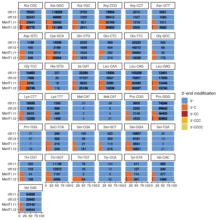
count_table_l %>%
mutate(rname = fct_relevel(rname,
sort(unique(as.character(rname)),
decreasing = FALSE)),
condition = fct_relevel(condition,
sort(unique(as.character(condition)),
decreasing = TRUE)),
downstream_seq = paste0("3'-", downstream_seq)) %>%
ggplot(aes(fill = downstream_seq, y = pc, x = condition)) +
geom_bar(position = "stack", stat = "identity") +
coord_flip() +
scale_fill_manual(values = palettefig) +
geom_text(aes(condition, 50, label = total, fill = NULL), size = 3) +
theme_classic() +
xlab(NULL) +
ylab(NULL) +
facet_wrap(facets = . ~ rname, ncol = 6, labeller = labeller(rname = labs)) +
labs(fill = "3'-end modification")
Differential proportion analysis: which tRNAs are significantly modified by toxin?
Are the observed differences in proportions of 3’-end modified transcripts statistically significant?
For this, we will compare the proportion of modified tRNAs in the conrtol vs. the proportion of modified tRNAs in the samples treated with MenT1.
In the following, we regroup the modified tRNAs as the “fraction” and we sum up unmodified and modified tRNAs in the “total” as expected by EMOTE_differential_proportion function.
proportion_table <- count_table_l %>%
  select(-rlength) %>%
  mutate(count_of = ifelse(downstream_seq == "", "total", "fraction")) %>%
  group_by(rname, strand, position, condition, count_of) %>%
  summarise(count = sum(count), .groups = "keep") %>%
  separate(condition, into = c("group", "replicate")) %>%
  pivot_wider(names_from = "count_of", values_from = "count", values_fill=0) %>%
  mutate(total = total + fraction) %>% # for dss which expects total and fraction
  pivot_longer(cols = c("fraction", "total"),
               names_to = "count_of",
               values_to = "count") %>%
  mutate(sample_id = paste0(group, ".", replicate, ".", count_of)) %>%
  select(-group, -replicate, -count_of)
proportion_table %>%
  head(15) %>%
  knitr::kable()
rname |
strand |
position |
count |
sample_id |
|---|---|---|---|---|
Msm.Ala-CGC.trna33 |
+ |
76 |
5891 |
MenT1.r1.fraction |
Msm.Ala-CGC.trna33 |
+ |
76 |
20841 |
MenT1.r1.total |
Msm.Ala-CGC.trna33 |
+ |
76 |
33505 |
MenT1.r2.fraction |
Msm.Ala-CGC.trna33 |
+ |
76 |
82775 |
MenT1.r2.total |
Msm.Ala-CGC.trna33 |
+ |
76 |
443 |
ctrl.r1.fraction |
Msm.Ala-CGC.trna33 |
+ |
76 |
75321 |
ctrl.r1.total |
Msm.Ala-CGC.trna33 |
+ |
76 |
79 |
ctrl.r2.fraction |
Msm.Ala-CGC.trna33 |
+ |
76 |
35347 |
ctrl.r2.total |
Msm.Ala-GGC.trna9 |
+ |
76 |
9965 |
MenT1.r1.fraction |
Msm.Ala-GGC.trna9 |
+ |
76 |
33503 |
MenT1.r1.total |
Msm.Ala-GGC.trna9 |
+ |
76 |
49391 |
MenT1.r2.fraction |
Msm.Ala-GGC.trna9 |
+ |
76 |
141388 |
MenT1.r2.total |
Msm.Ala-GGC.trna9 |
+ |
76 |
493 |
ctrl.r1.fraction |
Msm.Ala-GGC.trna9 |
+ |
76 |
118259 |
ctrl.r1.total |
Msm.Ala-GGC.trna9 |
+ |
76 |
83 |
ctrl.r2.fraction |
Then, we need a design_matrix to specify the group and replicate for each sample_id and also if the counts in the count_table corresponds to the fraction or the total.
design_matrix <- tibble(sample_id = unique(sort(proportion_table$sample_id))) %>%
  separate(sample_id,
           sep = "\\.",
           into = c("group", "replicate", "count_of"),
           remove = FALSE)
design_matrix %>%
  knitr::kable()
sample_id |
group |
replicate |
count_of |
|---|---|---|---|
ctrl.r1.fraction |
ctrl |
r1 |
fraction |
ctrl.r1.total |
ctrl |
r1 |
total |
ctrl.r2.fraction |
ctrl |
r2 |
fraction |
ctrl.r2.total |
ctrl |
r2 |
total |
MenT1.r1.fraction |
MenT1 |
r1 |
fraction |
MenT1.r1.total |
MenT1 |
r1 |
total |
MenT1.r2.fraction |
MenT1 |
r2 |
fraction |
MenT1.r2.total |
MenT1 |
r2 |
total |
diff_prop <- differential_proportion(proportion_table,
                                     design_matrix,
                                     group1 = "ctrl",
                                     group2 = "MenT1")
#> Estimating dispersion for each CpG site, this will take a while ...
diff_prop %>%
  knitr::kable()
rname |
position |
strand |
ctrl |
MenT1 |
pval |
fdr |
|---|---|---|---|---|---|---|
Msm.Gly-TCC.trna14 |
74 |
+ |
0.0079261 |
0.4145317 |
0.0000000 |
0.0000000 |
Msm.Cys-GCA.trna44 |
74 |
+ |
0.0044360 |
0.3793868 |
0.0000000 |
0.0000000 |
Msm.Arg-CCG.trna18 |
76 |
+ |
0.0020238 |
0.3288844 |
0.0000000 |
0.0000000 |
Msm.Ala-GGC.trna9 |
76 |
+ |
0.0029674 |
0.3233828 |
0.0000000 |
0.0000000 |
Msm.Arg-CCT.trna20 |
76 |
+ |
0.0009950 |
0.2765248 |
0.0000000 |
0.0000000 |
Msm.Leu-CAA.trna42 |
77 |
+ |
0.0014642 |
0.2638804 |
0.0000000 |
0.0000001 |
Msm.Leu-CAG.trna3 |
86 |
+ |
0.0013089 |
0.2679313 |
0.0000000 |
0.0000002 |
Msm.Tyr-GTA.trna4 |
86 |
+ |
0.0000000 |
0.2921362 |
0.0000001 |
0.0000002 |
Msm.Asp-GTC.trna31 |
77 |
+ |
0.0004209 |
0.2480578 |
0.0000002 |
0.0000009 |
Msm.Leu-GAG.trna13 |
89 |
+ |
0.0028787 |
0.2463040 |
0.0000002 |
0.0000009 |
Msm.Ala-TGC.trna2 |
76 |
+ |
0.0009452 |
0.2259275 |
0.0000003 |
0.0000010 |
Msm.Ala-CGC.trna33 |
76 |
+ |
0.0040582 |
0.3437180 |
0.0000005 |
0.0000016 |
Msm.SeC-TCA.trna46 |
95 |
+ |
0.0025000 |
0.2309671 |
0.0000018 |
0.0000052 |
Msm.Thr-GGT.trna5 |
76 |
+ |
0.0009011 |
0.2294034 |
0.0000039 |
0.0000103 |
Msm.Lys-CTT.trna17 |
76 |
+ |
0.0014216 |
0.1819812 |
0.0000053 |
0.0000131 |
Msm.Pro-GGG.trna41 |
77 |
+ |
0.0024442 |
0.2546503 |
0.0000060 |
0.0000138 |
Msm.Lys-TTT.trna21 |
76 |
+ |
0.0009772 |
0.1889863 |
0.0000068 |
0.0000149 |
Msm.Ser-GGA.trna24 |
89 |
+ |
0.0009599 |
0.2549558 |
0.0000135 |
0.0000277 |
Msm.Pro-CGG.trna23 |
77 |
+ |
0.0007758 |
0.1714434 |
0.0000150 |
0.0000293 |
Msm.Thr-TGT |
75 |
+ |
0.0000000 |
0.2202381 |
0.0000180 |
0.0000333 |
Msm.Glu-TTC.trna30 |
76 |
+ |
0.0010123 |
0.2098397 |
0.0000256 |
0.0000450 |
Msm.Gln-CTG.trna10 |
75 |
+ |
0.0025565 |
0.1654189 |
0.0000555 |
0.0000934 |
Msm.Asn-GTT.trna37 |
76 |
+ |
0.0009098 |
0.1908387 |
0.0000634 |
0.0001021 |
Msm.Ile-GAT.trna1 |
77 |
+ |
0.0010778 |
0.1727051 |
0.0001006 |
0.0001551 |
Msm.Thr-CGT.trna29 |
76 |
+ |
0.0015625 |
0.1889012 |
0.0001962 |
0.0002904 |
Msm.Val-CAC.trna12 |
75 |
+ |
0.0015707 |
0.1457437 |
0.0002308 |
0.0003284 |
Msm.Val-GAC.trna45 |
75 |
+ |
0.0010982 |
0.1332617 |
0.0002644 |
0.0003624 |
Msm.Gly-GCC.trna43 |
76 |
+ |
0.0000000 |
0.1832386 |
0.0003323 |
0.0004391 |
Msm.His-GTG.trna16 |
76 |
+ |
0.0000000 |
0.1934866 |
0.0009273 |
0.0011831 |
Msm.Ser-CGA.trna28 |
91 |
+ |
0.0000000 |
0.1653512 |
0.0011126 |
0.0013722 |
Msm.Glu-CTC.trna11 |
76 |
+ |
0.0000000 |
0.1664309 |
0.0042341 |
0.0050001 |
Msm.Ser-GCT.trna26 |
92 |
+ |
0.0000000 |
0.1193467 |
0.0043244 |
0.0050001 |
Msm.Met-CAT.trna6 |
77 |
+ |
0.0000000 |
0.0000000 |
0.7403609 |
0.8218854 |
Msm.Met-CAT.trna8 |
77 |
+ |
0.0000000 |
0.0000000 |
0.8104833 |
0.8218854 |
Msm.Pro-TGG.trna36 |
77 |
+ |
0.0000000 |
0.0000000 |
0.8057931 |
0.8218854 |
Msm.Ser-TGA.trna25 |
90 |
+ |
0.0000000 |
0.0000000 |
0.8115274 |
0.8218854 |
Msm.Trp-CCA.trna7 |
76 |
+ |
0.0000000 |
0.0000000 |
0.8218854 |
0.8218854 |
Notebook rendering time and memory:
time_end <- now()
rendering_time <- time_end - time_start
rendering_time
#> Time difference of 3.92412 mins
pryr::mem_used()
#> 1.56 GB