TSS identification using 5’-end RNA-Seq data

Complete source of this page is available in the notebook TSS_identification.Rmd.

library(tidyverse)

library(rnaends)

Based on the publication from Prados J, Linder P, Redder P (2016) TSS-EMOTE, a refined protocol for a more complete and less biased global mapping of transcription start sites in bacterial pathogens. BMC Genomics, 17, 849. https://doi.org/10.1186/s12864-016-3211-3.

The library preparation protocol is as follows. Briefly, in this protocol, total RNA is purified and digested with a 5’-exonuclease which removes the vast majority of 5’ mono-phosphorylated RNAs. The RNA is mixed with a synthetic RNA oligo (specific adapter) and split into two pools. In the first pool (noted +RppH), both a ligase and an RNA 5’ pyrophosphohydrolase RppH enzymes are added, while in the second pool (labeled -RppH) only the ligase is added. RppH converts the 5’PPP to 5’P that can be used by the ligase to add the adapter oligo to the RNA sequences (for detailed protocol see (Prados et al., 2016)). The “-RppH” pool serves as control to measure the level of background ligation and avoid false positive TSS detection. Thus, a given genome position will be predicted as a TSS if the number of reads from the “+RppH” pool mapping at that position is significantly higher than the number of reads from the “-RppH” pool by applying a beta-binomial test as described in (Prados et al., 2016)

Download datasets

Data from this article are available on Gene Expression Omnibus (GEO) database: https://www.ncbi.nlm.nih.gov/geo/query/acc.cgi?acc=GSE85110

For this notebook, only 4 samples will be used that correspond to 5’-end RNA-Seq data from Staphylococcus aureus (MW2 strain) grown on RPMI liquid at 37°C (GSM2257851, GSM2257852, GSM2257859, GSM2257860).

We download data directly in a the data directory of the GitLab project in the sub-directory called TSS-EMOTE_Prados where the reference genome is already provided when the project is cloned.

options(timeout = 3600) # for download time, set more if timeout occurs

list_SRR <- c("SRR3994381", "SRR3994382", "SRR3994390", "SRR3994389")

for (i in list_SRR){
    raw_fastq <- paste0("../extdata/TSS-EMOTE_Prados/", i, ".fastq.gz")
    if (!file.exists(raw_fastq))
        download.file(paste0("https://trace.ncbi.nlm.nih.gov/Traces/sra-reads-be/fastq?acc=",i),
                      destfile = raw_fastq)
}

Pre-processing of 5’-end RNA-Seq reads

Parse reads (+ read features)

Reads are not ready-to-map yet since they still have an adapter (the RP6 oligonucleotide) located at the 5’-end of each read.

We use parse_reads, in order to check that each read contains the expected elements in the adapter, the remove this oligonucleotide from the reads (see RP6 oligo TSS-EMOTE).

parse_reads requires a read_features table which defines the expected elements on the read.

Following the Materials & Methods section of the article, the structure of the reads can be schematized as follows (X is the mappable part):

      1       2            5      6            20     21    27      28 30     31                  50
      N     - (EMOTE barcode) -   CGGCACCAACCGAGG    - VVVVVVV -     CGC     - XXXXXXXXXXXXXXXXXXXXX
1 random nt -  EMOTE barcode  -   recognition.seq    -   UMI   - control.seq -     RNA 5'-end

We use init_read_features and add_read_feature functions to create the read_features table following the above structure.

The initialization of the read_features table is made by init_read_features since the only required feature is the readseq feature (the mappable part to keep in the FASTQ file).

According to our scheme, we know that the readseq part begins at location 31 and are 20 nucleotides long (illumina 50bp).

rf <- init_read_features(start = 31, width = 20)

We add other features such as the barcode which begins at position 2 and are 4 bases long with the following specifications:

pattern : enables to specify which barcode sequence(s) are allowed, here we allowed 4 different sequences
pattern_type: is used to know which type of pattern it is, “constant” means that we check the exact pattern sequences allowing N number of mismatches (specified by the max_mismatch parameter)
readid_prepend: is used to store the retrieved feature in the read identifier. It will be useful to keep a track of features since they are removed from the reads and therefore absent from the FASTQ output file.

rf <- add_read_feature(rf,
                       name = "barcode",
                       start = 2,
                       width = 4,
                       pattern = c("TCGG","CAAG","CGTC","AAGT"),
                       pattern_type = "constant",
                       max_mismatch = 0,
                       readid_prepend = FALSE)

The recognition sequence feature begins at position 6 and is 15 bases long, and we expect a single unique sequence with maximum 1 mismatch:

rf <- add_read_feature(rf,
                       name = "RS",
                       start = 6,
                       width = 15,
                       pattern = "CGGCACCAACCGAGG",
                       pattern_type = "constant",
                       max_mismatch = 1,
                       readid_prepend = FALSE)

The UMI feature begins at position 21 and is 7 bases long. Its pattern type is different from the previous ones because: as UMIs are random sequences, we do not expect a particular sequence (nor list of sequences) but a sequence of random characters (A, C or G) hence the patern_type = “nucleotides”. We set readid_prepend = TRUE because we will need the UMIs to remove PCR duplicates introduced by the library preparation protocol.

Note: the readseq feature has the same pattern_type than UMI and is set by default to A,C,T or G.

rf <- add_read_feature(rf,
                       name = "UMI",
                       start = 21,
                       width = 7,
                       pattern = "ACG",
                       pattern_type = "nucleotides",
                       max_mismatch = 0,
                       readid_prepend = TRUE)

The control sequence feature begins at position 28 and is 3 bases long, and we expect a specific and unique sequence:

rf <- add_read_feature(rf,
                       name = "CS",
                       start = 28,
                       width = 3,
                       pattern = "CGC",
                       pattern_type = "constant",
                       max_mismatch = 0,
                       readid_prepend = FALSE)

The resulting read_features table is:

rf %>%
  knitr::kable()

name	start	width	pattern_type	pattern	max_mismatch	readid_prepend
readseq	31	20	nucleotides	ACTG	0	FALSE
barcode	2	4	constant	TCGG, CA….	0	FALSE
RS	6	15	constant	CGGCACCA….	1	FALSE
UMI	21	7	nucleotides	ACG	0	TRUE
CS	28	3	constant	CGC	0	FALSE

Now that we have built the read_features table, we can parse the 4 FASTQ files with the parse_reads function.

Note: mclapply function from the parallel package is used to perform all the 4 processing in parallel but lapply can be used instead.

parsing_report <- lapply(
    list.files("../extdata/TSS-EMOTE_Prados/", pattern = ".fastq.gz$", full.names = TRUE),
    FUN = parse_reads,
    features = rf, # The read_features table
    keep_invalid_reads = FALSE, # do not store invalid reads
    out_dir = "../extdata/TSS-EMOTE_Prados/parse_results", # Path of the out directory (optional)
    force = FALSE
)
#> Demux report already exists set force=T to overwrite: ../extdata/TSS-EMOTE_Prados/parse_results/SRR3994381_parse_report.csv
#> Demux report already exists set force=T to overwrite: ../extdata/TSS-EMOTE_Prados/parse_results/SRR3994382_parse_report.csv
#> Demux report already exists set force=T to overwrite: ../extdata/TSS-EMOTE_Prados/parse_results/SRR3994389_parse_report.csv
#> Demux report already exists set force=T to overwrite: ../extdata/TSS-EMOTE_Prados/parse_results/SRR3994390_parse_report.csv

parsing_report %>%
  bind_rows %>%
  knitr::kable()

is_valid_readseq	is_valid_barcode	is_valid_RS	is_valid_UMI	is_valid_CS	count
FALSE	FALSE	TRUE	TRUE	FALSE	1
FALSE	TRUE	TRUE	TRUE	TRUE	1444
TRUE	FALSE	FALSE	TRUE	FALSE	272
TRUE	FALSE	TRUE	TRUE	FALSE	2668
TRUE	TRUE	TRUE	TRUE	TRUE	5189855
FALSE	FALSE	FALSE	TRUE	FALSE	3
FALSE	FALSE	TRUE	TRUE	FALSE	3
FALSE	TRUE	TRUE	TRUE	TRUE	2565
TRUE	FALSE	FALSE	TRUE	FALSE	3166
TRUE	FALSE	TRUE	TRUE	FALSE	21274
TRUE	TRUE	TRUE	TRUE	FALSE	1320
TRUE	TRUE	TRUE	TRUE	TRUE	8561052
FALSE	FALSE	FALSE	TRUE	FALSE	4
FALSE	TRUE	TRUE	TRUE	TRUE	2378
TRUE	FALSE	FALSE	TRUE	FALSE	2789
TRUE	FALSE	TRUE	TRUE	FALSE	1308
TRUE	TRUE	TRUE	TRUE	TRUE	3177298
FALSE	FALSE	FALSE	TRUE	FALSE	1
FALSE	FALSE	TRUE	TRUE	FALSE	1
FALSE	TRUE	TRUE	TRUE	TRUE	2876
TRUE	FALSE	FALSE	TRUE	FALSE	2924
TRUE	FALSE	TRUE	TRUE	FALSE	1237
TRUE	TRUE	TRUE	TRUE	TRUE	3774778

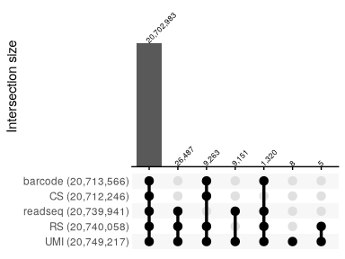
The parsing_report provides information on the validity of reads in each FASTQ file.

We can aggregate and visualize the global statititics for all reports with an upset plot:

parsing_report %>%
  bind_rows %>%
  group_by(across(starts_with("is_valid_"))) %>%
  summarise(count = sum(count), .groups = "drop") %>%
  reads_parse_report_ggupset(angle = 45, margin=0.3)

Quantification

Mapping

Reads are now ready-to-map on the reference genome using the map_fastq_files function.

Note: here, we use the function that allow the mapping of multiple FASTQ files in parallel which is a wrapper that calls the map_fastq function for each of the FASTQ files provided.

bf <- map_fastq_files(
  list_fastq_files = list.files("../extdata/TSS-EMOTE_Prados/parse_results", 
                                pattern = "_valid.fastq.gz$", 
                                full.names = TRUE),
  index_name = "../extdata/TSS-EMOTE_Prados/MW2.sr", # Path of the genome index (created if not exists)
  fasta_name = "../extdata/TSS-EMOTE_Prados/MW2.fasta", # Path of the reference genome file
  bam_dir = "../extdata/TSS-EMOTE_Prados/mapping_results_subread", # Output directory
  max_map_mismatch = 1,
  aligner = "subread", # either bowtie or subread
  map_unique = FALSE,
  force = FALSE,
  threads = 3)
#> bam_file '../extdata/TSS-EMOTE_Prados/mapping_results_subread/SRR3994381_valid.fastq.gz.bam' already exists, set force=TRUE to recompute
#> bam_file '../extdata/TSS-EMOTE_Prados/mapping_results_subread/SRR3994382_valid.fastq.gz.bam' already exists, set force=TRUE to recompute
#> bam_file '../extdata/TSS-EMOTE_Prados/mapping_results_subread/SRR3994389_valid.fastq.gz.bam' already exists, set force=TRUE to recompute
#> bam_file '../extdata/TSS-EMOTE_Prados/mapping_results_subread/SRR3994390_valid.fastq.gz.bam' already exists, set force=TRUE to recompute
bf
#> [[1]]
#> [1] "../extdata/TSS-EMOTE_Prados/mapping_results_subread/SRR3994381_valid.fastq.gz.bam"
#> 
#> [[2]]
#> [1] "../extdata/TSS-EMOTE_Prados/mapping_results_subread/SRR3994382_valid.fastq.gz.bam"
#> 
#> [[3]]
#> [1] "../extdata/TSS-EMOTE_Prados/mapping_results_subread/SRR3994389_valid.fastq.gz.bam"
#> 
#> [[4]]
#> [1] "../extdata/TSS-EMOTE_Prados/mapping_results_subread/SRR3994390_valid.fastq.gz.bam"

Mapping statistics

Use the map_stats_bam_files function to get some basic statistics on the mapping we’ve just performed:

map_stats_bam_files(bam_files = bf) %>%
  knitr::kable()
#> BAM file mapping stats exists '../extdata/TSS-EMOTE_Prados/mapping_results_subread/SRR3994381_valid.fastq.gz.bam.map_stats.csv' already exists, set force=TRUE to recompute
#> BAM file mapping stats exists '../extdata/TSS-EMOTE_Prados/mapping_results_subread/SRR3994382_valid.fastq.gz.bam.map_stats.csv' already exists, set force=TRUE to recompute
#> BAM file mapping stats exists '../extdata/TSS-EMOTE_Prados/mapping_results_subread/SRR3994389_valid.fastq.gz.bam.map_stats.csv' already exists, set force=TRUE to recompute
#> BAM file mapping stats exists '../extdata/TSS-EMOTE_Prados/mapping_results_subread/SRR3994390_valid.fastq.gz.bam.map_stats.csv' already exists, set force=TRUE to recompute

bam_file	mapped	unmapped	pc_mapped
SRR3994381_valid.fastq.gz.bam	2001012	3188843	38.56
SRR3994382_valid.fastq.gz.bam	3436440	5124612	40.14
SRR3994389_valid.fastq.gz.bam	781940	2395358	24.61
SRR3994390_valid.fastq.gz.bam	1433740	2341038	37.98

Quantification (counts computation)

In order to obtain counts per position, we use the quantify_from_bam_files function to parse previously obtained bam_files.

This function allows the quantification of either the 5’-ends (quantify_5prime) or the 3’-ends (quantify_3prime), in both cases, it is an exact position quantification.

For UMIs to be taken into account for the quantification, we provide the read_features table with the “features” parameter. The keep_UMI parameter is used to record the number of copy of each UMI by exact position. This level of information is not needed for this analysis and we use it as default (FALSE).

count_table <- quantify_from_bam_files(bam_files = bf,
                                       sample_ids = c("rep1-", "rep1+", "rep2-", "rep2+"),
                                       fun = quantify_5prime, # Either quantify_5prime or quantify_3prime
                                       features = rf,
                                       keep_UMI = FALSE)
#> Quantification 5' output file exists, set force=T to overwrite: ../extdata/TSS-EMOTE_Prados/mapping_results_subread/SRR3994381_valid.fastq.gz.bam.csv
#> Quantification 5' output file exists, set force=T to overwrite: ../extdata/TSS-EMOTE_Prados/mapping_results_subread/SRR3994382_valid.fastq.gz.bam.csv
#> Quantification 5' output file exists, set force=T to overwrite: ../extdata/TSS-EMOTE_Prados/mapping_results_subread/SRR3994389_valid.fastq.gz.bam.csv
#> Quantification 5' output file exists, set force=T to overwrite: ../extdata/TSS-EMOTE_Prados/mapping_results_subread/SRR3994390_valid.fastq.gz.bam.csv
count_table %>% 
  head(15) %>%
  knitr::kable()

sample_id	rname	position	strand	reads	count
rep1-	NC_003923.1	313	+	2	2
rep1-	NC_003923.1	425	+	34	9
rep1-	NC_003923.1	535	+	11	1
rep1-	NC_003923.1	637	+	1	1
rep1-	NC_003923.1	689	+	1	1
rep1-	NC_003923.1	791	+	2	1
rep1-	NC_003923.1	868	+	2	2
rep1-	NC_003923.1	911	+	2	1
rep1-	NC_003923.1	918	+	6	1
rep1-	NC_003923.1	1009	+	3	1
rep1-	NC_003923.1	1166	+	2	1
rep1-	NC_003923.1	1309	+	10	1
rep1-	NC_003923.1	1310	+	3	1
rep1-	NC_003923.1	1357	-	1	1
rep1-	NC_003923.1	1890	+	1	1

The above count table will allow us to perform some downstream analysis, i.e. TSS identification.

Note: here, the count column corresponds to the number of different UMIs mapped at this exact position. This is why it is lower or equal to the reads values (due to PCR duplicates).

Downstream analysis: TSS identification

Design table

The identification of TSS requires the comparison of 5’P and 5’P+5’PPP samples with multiple replicates. We thus build a design table to identify which samples is what.

The content of the design table is free as it includes the colnames:

sample_id (same as in the count table)
pool (library preparation for sequencing either “mono” for 5’P or “total” for 5’P+5’PPP)
replicate (p-values are combined by replicate)

design_tb <- tibble(
  sample_id = c("rep1-", "rep1+", "rep2-", "rep2+"),
  count_of = c("fraction", "total", "fraction", "total" ),
  replicate = c(1, 1, 2, 2)
)
design_tb %>%
  knitr::kable()

sample_id	count_of	replicate
rep1-	fraction	1
rep1+	total	1
rep2-	fraction	2
rep2+	total	2

Identification of TSS

We finally use the betabinom_TSS function to identify TSSs with the count table and the design table freshly built as inputs.

Note: the filtering of data is made by the function (and not before) because it needs the total number of counts before filtering.

bbin <- TSS(count_table = count_table,
            design_table = design_tb,
            threshold = 5, # Number minimum reads allowed in the total sample
            combine_method = "fisher", # Method for the p-values combination
            fdr_method = "fdr" # Method for adjusting p-value (see p.adjust)
            )
bbin %>% 
  head(15) %>%
  knitr::kable()

rname	position	strand	pvalue	pvalue_adj
NC_003923.1	312	+	0.0017109	0.0071046
NC_003923.1	313	+	0.0000000	0.0000000
NC_003923.1	314	+	0.0000001	0.0000008
NC_003923.1	1642	+	0.0725677	0.1682600
NC_003923.1	2131	+	0.0001241	0.0006330
NC_003923.1	3649	+	0.0000009	0.0000058
NC_003923.1	3650	+	0.0000000	0.0000000
NC_003923.1	3652	+	0.0000001	0.0000006
NC_003923.1	4128	+	0.0025859	0.0103542
NC_003923.1	4159	-	0.0000194	0.0001102
NC_003923.1	4301	+	0.1746218	0.3408392
NC_003923.1	6734	+	0.0182064	0.0576161
NC_003923.1	10687	-	0.0000000	0.0000000
NC_003923.1	10855	+	0.0000004	0.0000030
NC_003923.1	10856	+	0.1536700	0.3042540

Number of TSSs identified with an adjusted p-value (FDR) < 0.01: 2677.

Clusters of TSS

As in the Prados et al. paper we can clusterise TSSs by regrouping those less than 5 nucleotides apart.

bbin <- bbin %>% 
  filter(pvalue_adj < 0.01) %>% 
  arrange(position) %>%
   mutate(cluster_id = cumsum(c(1, diff(position) >= 5)))
bbin %>%
  head(15) %>%
  knitr::kable()

rname	position	strand	pvalue	pvalue_adj	cluster_id
NC_003923.1	312	+	0.0017109	0.0071046	1
NC_003923.1	313	+	0.0000000	0.0000000	1
NC_003923.1	314	+	0.0000001	0.0000008	1
NC_003923.1	2131	+	0.0001241	0.0006330	2
NC_003923.1	3649	+	0.0000009	0.0000058	3
NC_003923.1	3650	+	0.0000000	0.0000000	3
NC_003923.1	3652	+	0.0000001	0.0000006	3
NC_003923.1	4159	-	0.0000194	0.0001102	4
NC_003923.1	10687	-	0.0000000	0.0000000	5
NC_003923.1	10855	+	0.0000004	0.0000030	6
NC_003923.1	12473	+	0.0000000	0.0000000	7
NC_003923.1	14672	+	0.0000634	0.0003335	8
NC_003923.1	15797	+	0.0000000	0.0000000	9
NC_003923.1	17356	+	0.0000000	0.0000000	10
NC_003923.1	17357	+	0.0000000	0.0000000	10

Number of cluster of TSSs identified with an adjusted p-value (fdr) < 0.01: 1923.