Co-translational exoribonucleolytic degradation profiling in A. thaliana using 5’ end RNA-Seq data
Complete source of this page is available in the notebook Degradation_profiling_At.Rmd.
library(tidyverse)
time_start <- now()
library(ggpubr)
library(rnaends)
Co-translational exoribonucleolytic degradation analysis using 5’-end RNA-Seq data
Based on the publication from Cheng-Yu Hou, Wen-Chi Lee, Hsiao-Chun Chou, Ai-Ping Chen, Shu-Jen Chou, and Ho-Ming Chen (2016) Global Analysis of Truncated RNA Ends Reveals New Insights into Ribosome Stalling in Plants, Plant Cell, https://doi.org/10.1105/tpc.16.00295.
Download datasets
Data generated from this article are available on Gene Expression Omnibus (GEO) database: GSE77549
For this notebook, we will only use one sample corresonding to inflorescences of wild-type Arabidopsis from which total RNA was extacted and isolated for PARE library construction and sequencing (GSM2253889).
The raw sequencing data are downloaded in the “extdata” directory of the GitLab project in the subdirectory “Athaliana_Hou” using the NCBI fasterq-dump tool from NCBI:
fasterq-dump SRR3143655 --outdir ../extdata/Athaliana_Hou
Pre-processing
Parse reads (+ read features)
In order to make reads mappable, we must only keep the first 20 nucleotides as mentionned in the Material&Methods of the original article.
This is done with the parse_read function that validates the sequence composition (only A, T, C and G), and extracts the mappable part into a new FASTQ file for mapping to the reference sequences.
parse_reads utilizes a read_features table that describes each element that should be found in the reads. In this case, there is only one read feature: the first 20 nucleotides of the reads.
rf <- init_read_features(start = 1, width = 20)
rf %>%
  knitr::kable()
name |
start |
width |
pattern_type |
pattern |
max_mismatch |
readid_prepend |
|---|---|---|---|---|---|---|
readseq |
1 |
20 |
nucleotides |
ACTG |
0 |
FALSE |
Now, we can use the parse_reads function on the raw reads FASTQ file using the read_features table as parameter:
parse_reads("../extdata/Athaliana_Hou/SRR3143655.fastq.gz",
            yieldsize = 1e6, # Number of reads parsed at each iteration
            features = rf, # The features table
            out_dir = "../extdata/Athaliana_Hou/parsed_reads",
            keep_invalid_reads = FALSE, # We don't want to store invalid reads
            force = FALSE,
) %>%
  knitr::kable()
is_valid_readseq |
count |
|---|---|
FALSE |
35864 |
TRUE |
56567785 |
We observe that, from the 56,603,649 total reads, only 35,864 were discarded, and we are left with more than 56 millions reads that can be used further.
Quantification
Reads are now ready to be aligned on the reference sequences using the map_fastq function.
Reference sequences
For exoribonucleolytic degradation analysis, and particularly for periodicity analysis, we need to map the read sequences to protein coding sequences. Moreover, to study the 5’ends of transcripts around the START and STOP codon, we also need the 5’UTR and the 3’UTR.
To perform this, we will use the data from the TAIR10 database, and more precisely the following files avaliable for download:
TAIR10_cdna_20101214: all TAIR10 cDNA sequences
TAIR10_5_utr_20101028 and TAIR10_3_utr_20101028: 5’ and 3’ UTR of each gene.
These files are availabe (gzipped) in the extdata/Athaliana_Hou/reference_sequences directory of the GitLab project.
Mapping to reference sequences
The map_fastq function is called with the reads preprocessed previously in SRR3143655_valid.fastq.gz and with the reference sequences (cDNAs). The bowtie aligner is specified. For the mapping, we specify that one mixmatch is allowed in the alignments, and that reads should map to a unique location (map_unique = TRUE).
bf <- map_fastq(
  "../extdata/Athaliana_Hou/parsed_reads/SRR3143655_valid.fastq.gz",
  index_name = "../extdata/Athaliana_Hou/reference_sequences/TAIR10_cdna_20101214.bt", # Path of the genome index (created if not exists)
  fasta_name = "../extdata/Athaliana_Hou/reference_sequences/TAIR10_cdna_20101214.gz", # Path of the reference genome file
  bam_dir = "../extdata/Athaliana_Hou/mapping_results", # Output directory
  max_map_mismatch = 1,
  aligner = "bowtie", # Either bowtie or subread
  map_unique = TRUE,
  force = FALSE,
  threads = 3
)
#> Warning in FUN(X[[i]], ...): Index directory already exists remove it if you
#> want to recreate it
Quantification
In order to obtain counts by position, we use the quantify_from_bam_files function to parse previously obtained BAM file in bf.
This function allows the quantification of either the 5’-ends (quantify_5prime) or the 3’-ends (quantify_3prime), in both cases, it is an exact position quantification.
count_table <- quantify_from_bam_files(
    bam_files = bf,
    sample_ids = c("inflorescence"),
    fun = quantify_5prime, # Either quantify_5prime or quantify_3prime
    features = rf,
    force = FALSE)
count_table %>%
  head(15) %>%
  knitr::kable()
sample_id |
rname |
position |
strand |
count |
|---|---|---|---|---|
inflorescence |
AT1G50920.1 |
1 |
+ |
1 |
inflorescence |
AT1G50920.1 |
2 |
+ |
2 |
inflorescence |
AT1G50920.1 |
7 |
+ |
1 |
inflorescence |
AT1G50920.1 |
8 |
+ |
2 |
inflorescence |
AT1G50920.1 |
12 |
+ |
2 |
inflorescence |
AT1G50920.1 |
22 |
+ |
1 |
inflorescence |
AT1G50920.1 |
27 |
+ |
1 |
inflorescence |
AT1G50920.1 |
30 |
+ |
1 |
inflorescence |
AT1G50920.1 |
36 |
+ |
1 |
inflorescence |
AT1G50920.1 |
37 |
+ |
1 |
inflorescence |
AT1G50920.1 |
46 |
+ |
1 |
inflorescence |
AT1G50920.1 |
47 |
+ |
1 |
inflorescence |
AT1G50920.1 |
59 |
+ |
1 |
inflorescence |
AT1G50920.1 |
60 |
+ |
1 |
inflorescence |
AT1G50920.1 |
68 |
+ |
1 |
The above count table will allow us to perform some downstream analysis.
Downstream analysis
Annotation table preparation
In order to retrieve the number of reads mapped on the CDSs, we need to have access to the position (start and stop) of these CDSs.
We will use the BioStrings library to load the TAIR10 FASTQ files, and determine the lengths of the 5’ and 3’ UTRs of the cDNAs.
library(Biostrings)
Load all reference sequences (cDNAs) from FASTA:
cdna_ref <- readDNAStringSet("../extdata/Athaliana_Hou/reference_sequences/TAIR10_cdna_20101214.gz")
Extract names from FASTA descriptions:
cdna <- cdna_ref %>%
  names %>%
  tibble(fa=.) %>%
  separate(fa, sep=" \\| ", into=c("rname", "symbols", "desc", "loc")) %>%
  mutate(len = str_extract(loc, "LENGTH=\\d+"),
         len = as.numeric(str_extract(len, "\\d+$")))
Then, we use 5’ and 3’ UTR FASTA files to determine their length, and thus the location of START and STOP codons on cDNAs:
utr5 <- readDNAStringSet("../extdata/Athaliana_Hou/reference_sequences/TAIR10_5_utr_20101028.gz")
utr5 <- utr5 %>%
  names %>%
  tibble(fa=.) %>%
  separate(fa, sep=" \\| ", into=c("rname", "ranges", "loc")) %>%
  mutate(utr5len = str_extract(loc, "LENGTH=\\d+"),
         utr5len = as.numeric(str_extract(utr5len, "\\d+$"))) %>%
  select(rname, utr5len)
Same on the 3’UTR:
utr3 <- readDNAStringSet("../extdata/Athaliana_Hou/reference_sequences/TAIR10_3_utr_20101028.gz")
utr3 <- utr3 %>%
  names %>%
  tibble(fa=.) %>%
  separate(fa, sep=" \\| ", into=c("rname", "ranges", "loc")) %>%
  mutate(utr3len = str_extract(loc, "LENGTH=\\d+"),
         utr3len = as.numeric(str_extract(utr3len, "\\d+$"))) %>%
  select(rname, utr3len)
We merge all the information in the cdna tibble:
cdna <- cdna %>%
  left_join(utr5, by = join_by(rname)) %>%
  left_join(utr3, by = join_by(rname)) %>%
  replace_na(list(utr5len = 0, utr3len=0))
And, we reformat these data into the annot table that will be used for analysing regions around features (START and STOP codons), and periodicity on the CDSs.
annot <- tibble(
  rname = cdna$rname,
  feature = "CDS",
  strand = "+",
  start = 1 + cdna$utr5len,
  end = cdna$len   - cdna$utr3len,
  annotation = names(cdna_ref)
)
annot %>%
  head(15) %>%
  knitr::kable()
rname |
feature |
strand |
start |
end |
annotation |
|---|---|---|---|---|---|
AT1G51370.2 |
CDS |
+ |
1 |
1041 |
AT1G51370.2 | Symbols: | F-box/RNI-like/FBD-like domains-containing protein | chr1:19045615-19046825 FORWARD LENGTH=1118 |
AT1G50920.1 |
CDS |
+ |
119 |
2134 |
AT1G50920.1 | Symbols: | Nucleolar GTP-binding protein | chr1:18870139-18872930 FORWARD LENGTH=2394 |
AT1G36960.1 |
CDS |
+ |
1 |
546 |
AT1G36960.1 | Symbols: | unknown protein; BEST Arabidopsis thaliana protein match is: unknown protein (TAIR:AT1G48095.1); Has 54 Blast hits to 54 proteins in 2 species: Archae - 0; Bacteria - 0; Metazoa - 0; Fungi - 0; Plants - 54; Viruses - 0; Other Eukaryotes - 0 (source: NCBI BLink). | chr1:14014796-14015508 FORWARD LENGTH=546 |
AT1G44020.1 |
CDS |
+ |
1 |
1734 |
AT1G44020.1 | Symbols: | Cysteine/Histidine-rich C1 domain family protein | chr1:16716112-16718656 REVERSE LENGTH=2314 |
AT1G15970.1 |
CDS |
+ |
375 |
1433 |
AT1G15970.1 | Symbols: | DNA glycosylase superfamily protein | chr1:5486319-5488868 REVERSE LENGTH=1658 |
AT1G73440.1 |
CDS |
+ |
56 |
820 |
AT1G73440.1 | Symbols: | calmodulin-related | chr1:27611363-27612815 FORWARD LENGTH=1453 |
AT1G75120.1 |
CDS |
+ |
147 |
1355 |
AT1G75120.1 | Symbols: RRA1 | Nucleotide-diphospho-sugar transferase family protein | chr1:28196857-28198802 REVERSE LENGTH=1520 |
AT1G17600.1 |
CDS |
+ |
93 |
3242 |
AT1G17600.1 | Symbols: | Disease resistance protein (TIR-NBS-LRR class) family | chr1:6052936-6056664 REVERSE LENGTH=3332 |
AT1G50860.1 |
CDS |
+ |
1 |
3846 |
AT1G50860.1 | Symbols: | transposable element gene | chr1:18850511-18854356 REVERSE LENGTH=3846 |
AT1G51380.1 |
CDS |
+ |
79 |
1257 |
AT1G51380.1 | Symbols: | DEA(D/H)-box RNA helicase family protein | chr1:19047882-19050162 FORWARD LENGTH=1452 |
AT1G77370.1 |
CDS |
+ |
74 |
466 |
AT1G77370.1 | Symbols: | Glutaredoxin family protein | chr1:29073843-29074796 FORWARD LENGTH=620 |
AT1G44090.1 |
CDS |
+ |
1 |
1158 |
AT1G44090.1 | Symbols: ATGA20OX5, GA20OX5 | gibberellin 20-oxidase 5 | chr1:16760677-16762486 REVERSE LENGTH=1158 |
AT1G10950.1 |
CDS |
+ |
114 |
1883 |
AT1G10950.1 | Symbols: TMN1, AtTMN1 | transmembrane nine 1 | chr1:3659209-3663984 FORWARD LENGTH=2245 |
AT1G31870.1 |
CDS |
+ |
161 |
1846 |
AT1G31870.1 | Symbols: | unknown protein; FUNCTIONS IN: molecular_function unknown; INVOLVED IN: biological_process unknown; LOCATED IN: cytosol, nucleus; EXPRESSED IN: 25 plant structures; EXPRESSED DURING: 15 growth stages; CONTAINS InterPro DOMAIN/s: Protein of unknown function DUF2050, pre-mRNA-splicing factor (InterPro:IPR018609); Has 13303 Blast hits to 9618 proteins in 489 species: Archae - 8; Bacteria - 444; Metazoa - 7153; Fungi - 2294; Plants - 942; Viruses - 128; Other Eukaryotes - 2334 (source: NCBI BLink). | chr1:11436747-11440109 FORWARD LENGTH=2134 |
AT1G51360.1 |
CDS |
+ |
25 |
657 |
AT1G51360.1 | Symbols: ATDABB1, DABB1 | dimeric A/B barrel domainS-protein 1 | chr1:19044184-19044900 FORWARD LENGTH=717 |
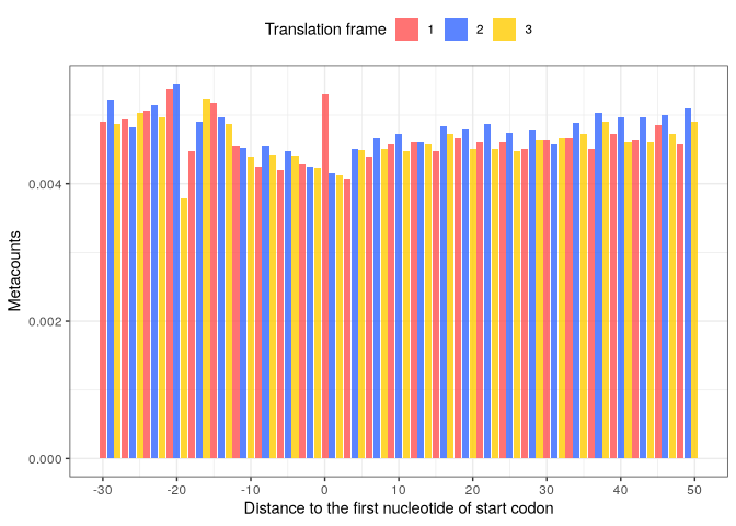
Metagene counts
Now that we have the count table and the annotation table, we can compute the metacount profiles around the first nucleotide of the START or STOP codon using the metacounts_feature function.
First, we extract the regions spanning around the feature (START or STOP codon) with metacounts_feature:
start_tb <- annot %>%
  select(rname, strand, position=start)
start_metacounts <- metacounts_feature(count_table, start_tb, width=100)
start_metacounts %>%
  head(15) %>%
  knitr::kable()
x |
count |
|---|---|
-100 |
0.0057777 |
-99 |
0.0058652 |
-98 |
0.0058652 |
-97 |
0.0060961 |
-96 |
0.0060172 |
-95 |
0.0056927 |
-94 |
0.0056102 |
-93 |
0.0056927 |
-92 |
0.0062604 |
-91 |
0.0057777 |
-90 |
0.0059554 |
-89 |
0.0055860 |
-88 |
0.0057777 |
-87 |
0.0059554 |
-86 |
0.0054522 |
Then, we can visualize the metacounts profile:
start_metacounts %>%
  plot(from = -30, to = 50,
       translation_frame = TRUE,
       geom = "bar",
       x_lab = "Distance to the first nucleotide of start codon")
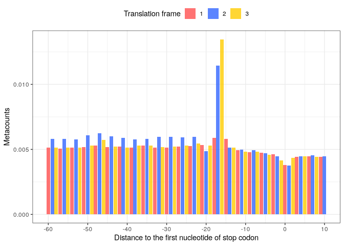
We perform the same for the STOP codon (adjusting for the position of the 1st nucleotide):
stop_tb <- annot %>%
  select(rname=rname, strand, position=end) %>%
  mutate(position = ifelse(strand=='+', position-2, position+2))
stop_metacounts <- metacounts_feature(count_table, stop_tb, width=100)
stop_metacounts %>%
  head(15) %>%
  knitr::kable()
x |
count |
|---|---|
-100 |
0.0049187 |
-99 |
0.0050808 |
-98 |
0.0057159 |
-97 |
0.0050104 |
-96 |
0.0048753 |
-95 |
0.0055718 |
-94 |
0.0050231 |
-93 |
0.0050231 |
-92 |
0.0057656 |
-91 |
0.0050692 |
-90 |
0.0049882 |
-89 |
0.0055718 |
-88 |
0.0050734 |
-87 |
0.0050614 |
-86 |
0.0056914 |
Metacount profile obtained:
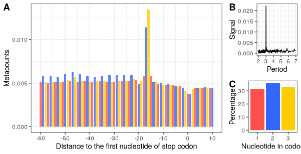
p_stop_metacounts <- stop_metacounts %>%
  plot(from = -60, to = 10,
       translation_frame = TRUE,
       geom = "bar",
       x_lab = "Distance to the first nucleotide of stop codon")
p_stop_metacounts
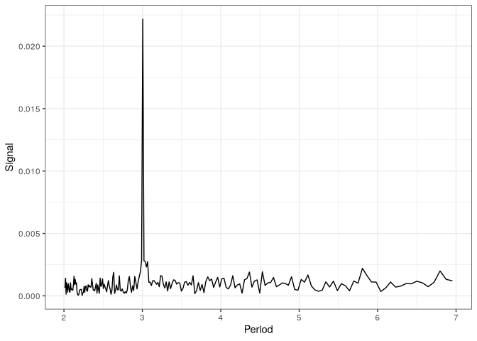
Periodicity
With the annotation table annot, we can compute the metacounts profile for all the CDS regions, and use FFT to analyse periodicity in the counts.
cds_tb <- annot %>%
  select(rname, strand, begin=start, end)
stop_tb <- annot %>%
  select(rname=rname, strand, position=end) %>%
  mutate(position = ifelse(strand=='+', position-2, position+2))
fft_tb <- FFT(count_table = count_table,
              region_tb = cds_tb)
fft_tb %>%
  head(15) %>%
  knitr::kable()
signal |
freq |
period |
|---|---|---|
0.0221807 |
199 |
3.005025 |
0.0049231 |
25 |
23.920000 |
0.0046483 |
24 |
24.916667 |
0.0045493 |
27 |
22.148148 |
0.0041448 |
28 |
21.357143 |
0.0038850 |
30 |
19.933333 |
0.0038517 |
26 |
23.000000 |
0.0035768 |
32 |
18.687500 |
0.0035188 |
29 |
20.620690 |
0.0035124 |
34 |
17.588235 |
0.0035022 |
31 |
19.290323 |
0.0034541 |
55 |
10.872727 |
0.0032312 |
39 |
15.333333 |
0.0031251 |
38 |
15.736842 |
0.0031005 |
37 |
16.162162 |
p_fft <- fft_tb %>%
  filter(period < 7) %>%
  plot()
p_fft
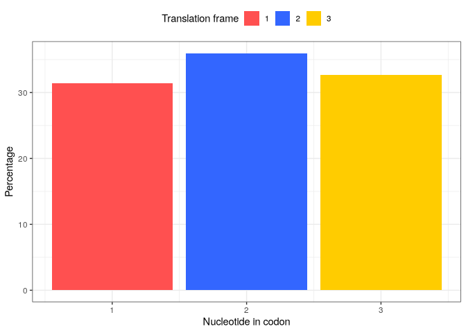
Frame preference
The third analysis provided in this downstream analysis is the count of reads falling into each translation frame (1, 2 or 3). The frame_preference function takes the same inputs as the 2 previous functions.
frame_pref_tb <- frame_preference(count_table = count_table,
                                  region_tb = cds_tb)
frame_pref_tb %>%
  knitr::kable()
frame |
pc |
|---|---|
1 |
31.38806 |
2 |
35.97309 |
3 |
32.63885 |
Visualisation
p_frame_pref <- plot(frame_pref_tb) +
  xlab("Nucleotide in codon")
p_frame_pref
Final plot:
library(ggpubr)
p1 <- p_stop_metacounts + theme(legend.position = "none")
p3 <- p_frame_pref + theme(legend.position = "none")
ggarrange(p1,
          ggarrange(p_fft, p3, nrow=2, labels = c("B","C")),
          widths = c(3,1),
          labels = c("A","")
)
Notebook rendering time and memory:
time_end <- now()
rendering_time <- time_end - time_start
rendering_time
#> Time difference of 15.94422 hours
pryr::mem_used()
#> 1.36 GB